Lately, there has been a shift in how foundation models operate.

After establishing that pretraining a large Deep Learning model on a vast corpus of temporal data grants generalizable properties, pretrained TS models now aim to be even more versatile.

For time series, this means supporting exogenous variables and allowing variable context and prediction lengths.

This article discusses Timer-XL[1], an upgraded time series model based on Timer[2]. Timer-XL is built for generalization, with a focus on long-context forecasting.

The model is open-source — I’ll also walk through a tutorial for univariate forecasting in Part 2!

Let’s get started!

✅ Find the 2 Timer-XL notebooks in the AI Projects folder (Project 18 and Project 19)

✅ 80% of paid subscribers have stayed for over a year since I launched. If you’re in it for the long run, consider switching to an annual subscription—you’ll save 23%!

Get the Annual subscription! 🎁

What is Time-XL

Key features of Timer-XL:

• Varying input/output lengths: Unlike models such as TTM that have various versions for different input or output lengths, Time-XL uses a single model for all cases, without making assumptions about context or prediction length.

• Long-context forecasting: Handles longer lookback windows effectively.

• Rich features: Forecasts non-stationary univariate series, complex multivariate dynamics, and covariate-informed contexts with exogenous variables — all in a unified setup.

• Versatile: Can be trained from scratch or pretrained on large datasets. Further finetuning is optional for improved performance.

Timer-XL enhances forecasting accuracy by introducing TimeAttention — an elegant attention mechanism that we’ll discuss in detail below.

The team behind Timer-XL (THUML lab at Tsinghua University[3]) has deep expertise in time-series modeling. They’ve released milestone models like iTransformer, TimesNet, and Timer — Timer-XL’s predecessor.

They also recently introduced Sundial — a foundation model excelling in probabilistic forecasting (we’ll explore it in a future article, so stay tuned!).

Encoder vs Decoder vs Encoder-Decoder models

Before discussing Timer-XL, we’ll explore the related work and recap the state of foundation TS models — this will help us understand what led to Timer-XL’s breakthrough.

NLP Applications

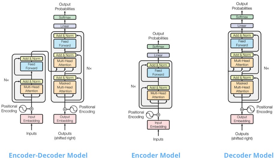
In the early days of the Transformer, there was debate over which architecture was most effective. The original Transformer was an Encoder-Decoder model.

Later, the Transformer research split into 2 branches: Encoder-only, like BERT (led by Google), and decoder-only, like GPT (led by OpenAI):

• Encoder-Decoder models use a bidirectional encoder to understand input and a causal decoder to generate output one token at a time. They excel at sequence-to-sequence tasks such as translation and summarization.

• Encoder-only models use bidirectional attention (look for context in both ways) to understand a sentence and predict masked words within a sentence. They excel at NLU (natural language understanding) tasks.

• Decoder-only models use causal attention (the model only looks back for context) and learn to predict the next word. They excel at NLG (natural language generation) tasks.

In NLP, decoder-only models dominate generation tasks. Encoder-only models are used in classification, regression, and NER (Named Entity Recognition).

Time-Series Applications

By late 2024 and early 2025, numerous foundation models were published, providing ample evidence of what works best.

All these foundation models have come in many flavours. Examples are:

• Decoder models

  • TimesFM (Google), Time-MOE

• Encoder models

  • MOIRAI (Salesforce), MOMENT

• Encoder-Decoder

  • Chronos (Amazon)

So far, decoder and encoder-decoder models outperform encoders in forecasting. Timer-XL’s authors back this up with extensive experiments — their results support the same conclusion.

There is also a category of multi-purpose models — used for forecasting, classification, imputation, etc. MOMENT and UNITS belong here and are encoder-only models.

Timer, also multi-purpose, is a decoder-only model. Its successor, Timer-XL, outperforms Timer in forecasting, but specializes in that task alone.

Therefore:

• For tasks that require general time-series understanding (e.g., imputation, anomaly detection), encoder models may be more suitable.

• However, for time-series forecasting, decoders currently hold the lead.

Long-Context Forecasting

The primary advantage of Transformer models is their ability to handle a large context length.

Modern LLMs such as Gemini support up to 1M tokens. They’re not flawless at this scale, but generally reliable up to 100k tokens.

Time-series models are far behind — Transformer and DL forecasting models often struggle beyond 1K tokens. Recent foundation models such as MOIRAI support up to 4K.

There are 2 issues to examine here:

• The maximum supported context length.

• How the model handles the increased context length, in terms of performance.

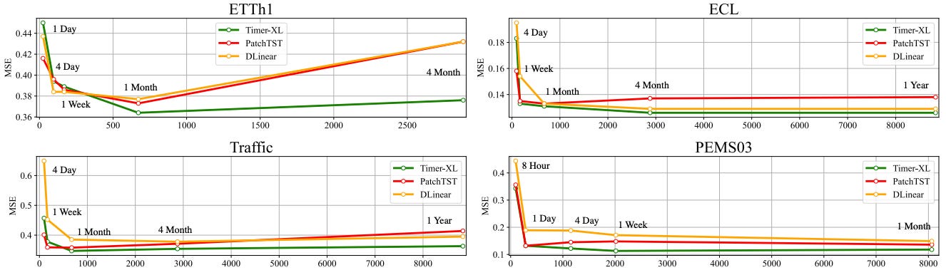
Figure 2 shows that Timer-XL handles increasing context better than other models.

For daily datasets such as Traffic, we can use up to a year’s data (~8760 datapoints). This makes Timer-XL ideal for high-frequency forecasting — a configuration where foundation models often underperform, as discussed earlier.

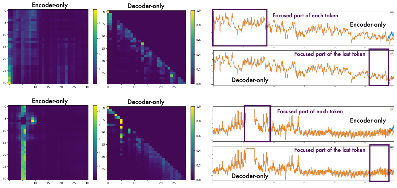
Since we previously discussed Encoder-vs-Decoder models, let’s mention how this paper explored how each architecture affects the efficiency of Long-Context Forecasting.

In Figure 3, they analyzed where the model focuses during prediction using attention maps:

Let’s interpret the above plots:

Encoder: Exhibits broad and diffuse attention across most of the sequence. Each token attends to many other tokens—this suggests less focus. Occasionally, they focus on irrelevant parts, completely missing the most recent datapoints.

Decoder: Sparse, triangular structure. Attention is mostly local and causal (as expected), but selective peaks suggest it occasionally “reaches back” further when useful.

TimeAttention: The “Secret Sauce” of Timer-XL

The attention mechanism powers the Transformer (a breakthrough in NLP), but in time series, it’s a double-edged sword. We discussed this extensively here.

In short:

1. Transformer Time Series models are prone to overfitting.

2. We cannot use raw attention as in NLP because self-attention is permutation-invariant (the order of tokens doesn’t matter, which it should when we have temporal information).

Let’s first examine how deep learning models address time series, focusing on SOTA methods from each year.

Preliminaries

In DL time series, a single data point or a patch (a group of consecutive data points) is referred to as a token.

Imagine a dataset of 3 time series, where y is the target variable and x, z are observed covariates. For an input size T, the sequences are formatted as:

• y1, y2, y3 … yT

• x1, x2, x3 … xT

• z1, z2, z3 … zT

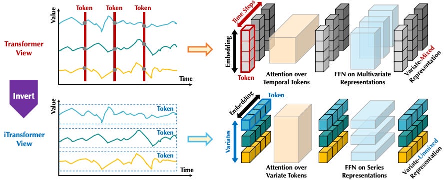
Early Transformer models like PatchTST applied attention across the time dimension, e.g., between <y1, x1, z1>, <y2, x2, z2> … <yN, xN, zN>.

This approach has a few disadvantages — e.g., misses lagged information across the feature dimension.

Later models, such as iTransformer, addressed this by applying attention across the feature/variate dimension, between <y1,y2,y3, … yN >, <x1,x2,x3, … xN >, <z1,z2,z3, … zN>. You can see the difference between the 2 approaches in Figure 4 below:

As you might have guessed, we can further improve performance by combining both approaches. For instance, CARD (an encoder-only model) employs a sequential 2-stage attention mechanism for cross-time, cross-feature dependencies (Figure 5):

However, this method is slow — due to its sequential 2-stage design.

MOIRAI took things to the next level by introducing Any-Variate Attention, a novel attention mechanism adapted for pretrained models.

Any-Variate captures temporal relationships among datapoints while preserving permutation invariance across covariates. We discussed this mechanism in detail here.

Next, we dive into Timer-XL’s TimeAttention.

Enter TimeAttention

MOIRAI is a masked encoder model, so Any-Variate Attention can’t be used as-is in decoder-only models like Timer-XL.

Decoder-only models use causal self-attention — attending only to previous tokens. In contrast, vanilla quadratic self-attention is bidirectional.

To address this, Timer-XL introduces a causal variant of MOIRAI’s attention called TimeAttention.

Specifically, TimeAttention introduces:

• Rotary positional embeddings (ROPE) to capture time dependencies

• Binary biases (ALIBI) to capture dependencies among variates.

• Causal self-attention.

The goal of TimeAttention is:

1. No permutation invariance for temporal information — the ordering of datapoints/temporal tokens should matter.

2. Permutation invariance between the variates/features — ordering of the variates should not matter (e.g., if we have 2 covariates X1 and X2, it does not matter which is first, just the relationship between them). This achieves permutation equivalence.

The attention score between the (m,i)-th query and the (n,j)-th key, where i,j represent the time indexes and (m,n) the variate indexes, is calculated as follows:

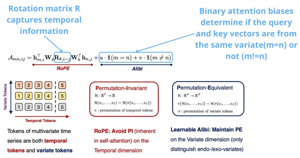
TimeAttention enables Timer-XL to handle univariate, multivariate, and context-informed forecasting.

Given N variables for a dataset, the model flattens the 2D input [observations, N] into 1D indices and calculates the attention-score by respecting permutation invariance in the time dimension and permutation equivariance in the variate dimension.

Standard self-attention is pairwise, resulting in quadratic cost. A key difference from MOIRAI is the use of causal attention, where each patch attends to previous points of its own signal, or to other time signals.

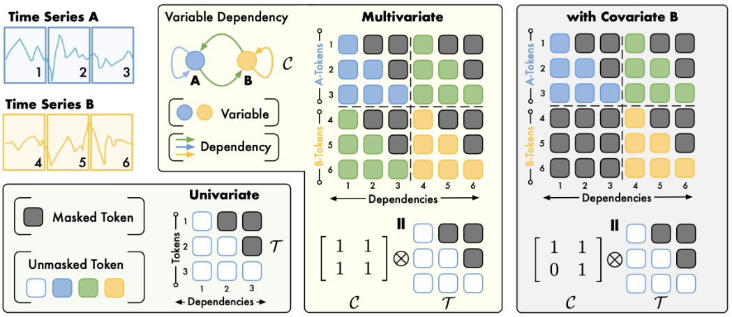
In Figure 7’s example, say we have 2 time series, A and B, each consisting of 3 tokens. The interactions are shown more clearly in Figure 8:

• Time Series A consists of tokens 1, 2, and 3

• Time Series A consists of tokens 4, 5, and 6

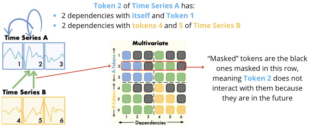
For Token 2 of Time Series A, the following attention scores are calculated:

• token2 ←→ token2 (to itself)

• token2 ←→ token1

• token2 ←→ token4

• token2 ←→ token5

The first 2 attention scores are within time series A, while the last 2 are within time series B. The TimeAttention formula can distinguish different time series and preserve permutation-equivalence.

While TimeAttention may seem complex and somewhat arbitrary, ablation studies performed by the authors show it offers optimal performance in this setup.

Note: When we mention tokens, we don’t mean individual datapoints. Timer-XL uses patches as tokens — so attention scores are computed between patches, not individual datapoints.

Enter Timer-XL

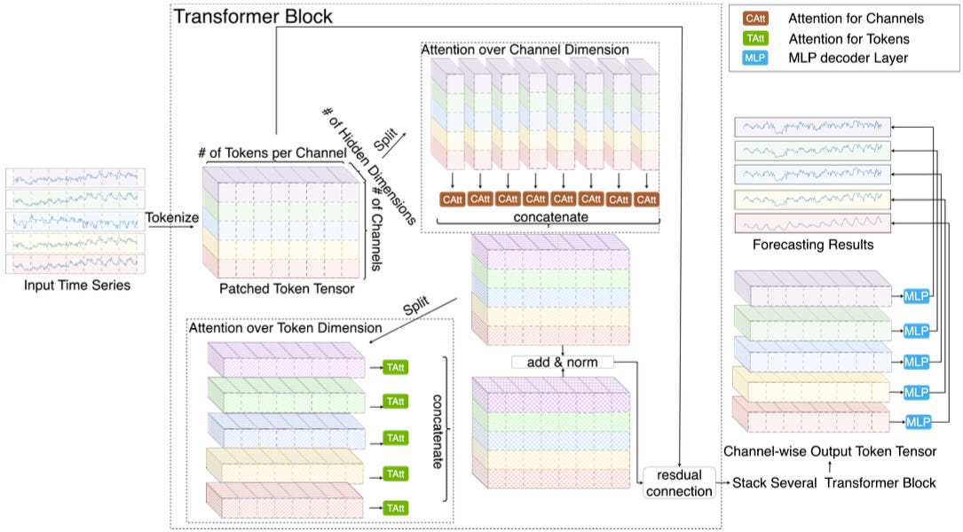
The full architecture of Timer-XL is shown below:

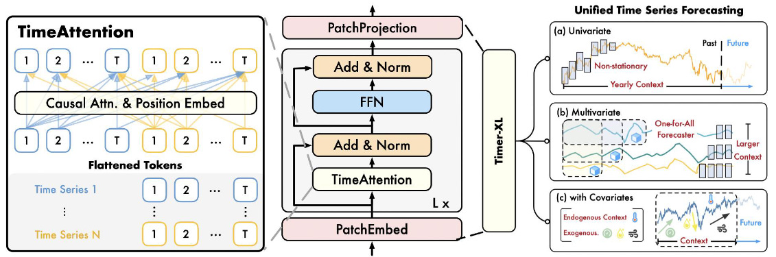
Timer-XL focuses on long-context and long-term forecasting using TimeAttention. Moreover, Timer-XL uses the latest perks of advanced LLMs like FlashAttention:

Interestingly, Timer-XL does not benefit from Reversible Instance Normalization (RevIN) — a technique often used to handle distribution shifts in time-series data. The authors attribute this to the window-centric structure of Timer-XL, which operates across different variates (likely due to the flattening process).

Let’s now check some interesting benchmarks!

Multivariate Forecasting Benchmark

Timer-XL is primarily a zero-shot foundation model, but it can also be trained from scratch on specific datasets.

In Table 1, Timer-XL is benchmarked against popular DL models across well-known datasets. For each dataset, average MAE and MSE are reported using a rolling-forecast evaluation across the test set.

Rolling Forecasting: In this approach, each model is trained with 672 input steps to produce N = (96, 192, 336, or 720) output steps. The previous window slice of real observations is then recursively fed back as input until the target forecast length N is reached. Table 1 shows the average score across all prediction lengths.

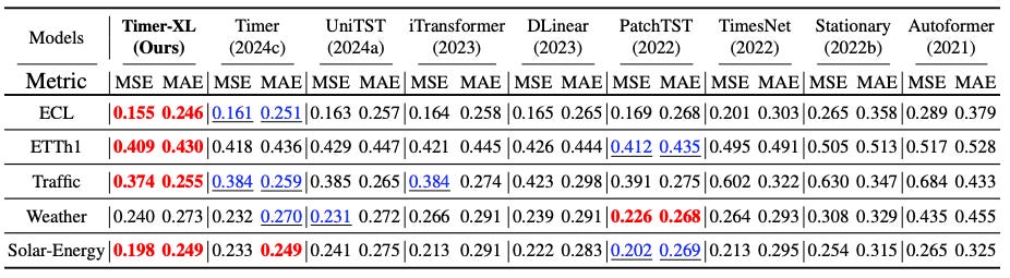
Key takeaways:

• Timer-XL achieves the best average scores.

• Previous SOTA models like PatchTST and iTransformer ranked among the top 2 in a few cases.

• Timer-XL and Timer — the only decoder-only models — perform the best.

The benchmark is further extended to include time-series models from other domains. Below are results from the GTWSF dataset (a wind speed forecasting challenge):

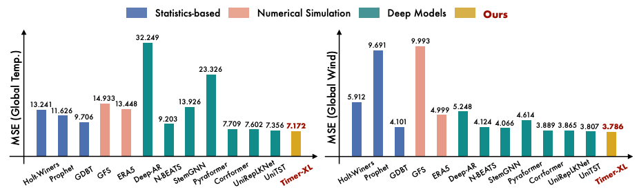
We observe:

• Timer-XL achieves the top overall score.

• Most DL models perform well, though some fail spectacularly!

• GDBT is not a statistics-based method, probably refers to Boosted Trees – in fact, it would be nice if the popular GDBT models like LightGBM were present here.

• A Seasonal Naive baseline would’ve been a useful inclusion as well.

Covariate-Informed Time Series Forecasting

In multivariate forecasting, each time series is treated as a separate channel. The model captures their inter-dependencies and jointly forecasts all time series.

In covariate-informed forecasting, we predict a target series using others as covariates. These may be past-observed, future-known, or static. That’s the setup discussed here.

An example of covariate-informed forecasting is shown in Figure 7 (right). In that case we predict variable A based on its dependency (green arrow) from B.

Table 2 shows results on the EPF dataset (electricity price forecasting task, Lago et al., 2021). The authors include both the current Timer-XL and an encoder Timer-XL variant (the one with the non-causal tag).

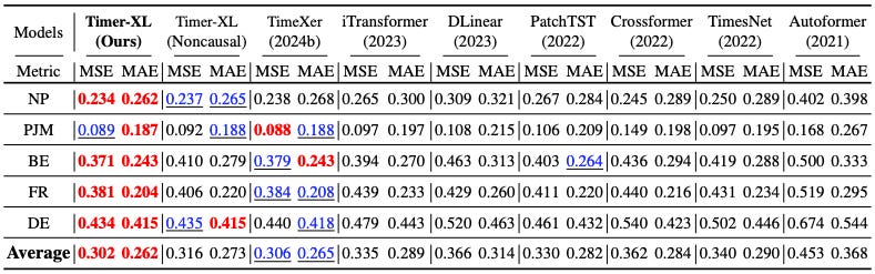
Observe that:

• Timer-XL achieves the best results.

• The decoder version (Timer-XL) outperforms the encoder-based Timer-XL.

• TimerXer is an encoder-based Transformer that uses cross-attention to model dependencies with exogenous variables, each treated as a separate token. This was a previous SOTA DL model — now outperformed by Timer-XL.

Zero-Shot Forecasting Benchmark

Finally, the authors also evaluate Timer-XL as a foundation model, comparing it with other top time series models.

They perform univariate pretraining on the LOTSA dataset (used to pretrain MOIRAI) and UTSD. The latter was curated by the THUML research group and used to pretrain Timer. It contains 1B datapoints.

The same metrics and configurations as before are used (e.g., scores averaged across prediction_lengths ={96, 192, 336, 720}). This time, none of the models were trained on the below datasets (zero-shot forecasting).

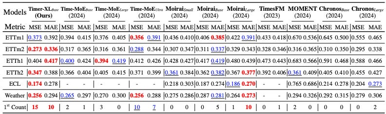
We notice the following:

• Timer-XL-base (the zero-shot version) scores the most wins.

• Time-MOE-ultra ranks 2nd, followed by the MOIRAI models.

• Interestingly, MOIRAI-Base takes some wins from MOIRAI-Large — a pattern seen in other benchmarks. Despite having fewer parameters, MOIRAI-Base often matches or outperforms MOIRAI-Large.

• Unfortunately, the SOTA versions of existing pretrained models are not included. For example, newer versions like TimesFM-2.0, Chronos-Bolt, MOIRAI-MOE, and other popular models, such as Tiny-Time-Mixers (TTM) and TabPFN-TS, are missing.

The authors have included the complete benchmark of foundation models in Table 13 of the paper. Feel free to read the paper for more details. In those results, I noticed that Timer-XL performs slightly better with longer prediction lengths compared to the other models.

Interpretability

Few time-series models explore interpretability, especially the DL models. Timer-XL authors demonstrate the benefits of attention by showing how it captures interdependencies among time series variables.

Figure 11 shows the average attention score across all attention matrices. The matrix is 10×10, which corresponds to the attention score pairs among 10 variables. The 2 tiles in the figure show the relationship between attention and correlation. The pair of variables <6,7> has a higher attention score than <6,2>—which correctly translates to the pair <6,7> having a higher correlation.

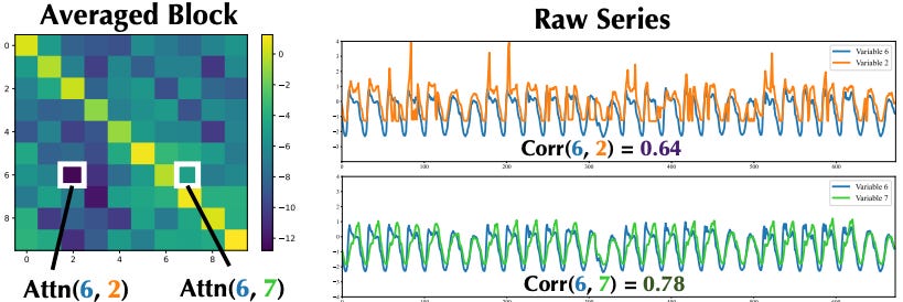
Hence, we conclude:

This isn’t a new pattern—we have seen many Transformer forecasting models using this trick. In this case, it means Timer-XL’s attention mechanism works as expected and correctly captures the variate dependencies.

Univariate Forecasting Tutorial

At the time of writing this article, the authors have released the univariate pretrained version of Timer-XL.

Thus, I used this version for now to evaluate Timer-XL on the ETTh2 dataset and the latest month of the SP&500 index.

The results are quite promising. Figure 12 shows Timer-XL’s predictions on the ETTh2 dataset:

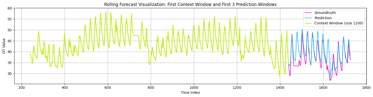
I don’t want to make this article very long, so we’ll go through the tutorials on Part 2. You can also find them in the AI Projects Folder (Project 18 and Project 19). Stay tuned!

Thank you for reading!

Horizon AI Forecast is a reader-supported newsletter, featuring occasional bonus posts for supporters. Your support through a paid subscription would be greatly appreciated.

Subscribe now

References

[1] Liu et al. Timer-XL: Long-context Transformers For Unified Time Series Forecasting (March 2025)

[2] Liu et al. Timer: Generative Pre-trained Transformers Are Large Time Series Models (October 2024)

[3] THUML @ Tsinghua University

[4] Liu et al. Timer-XL ICRL2025 Presentation Slides

AI Horizon Forecast