The recent release of Llama 4 [1] was far from perfect, but there is a lot that can be learned from this new generation of models. Put simply, Llama 4 is a massive pivot in Meta’s research direction. In response to increasing competition, Meta is reinventing the Llama series and clearly pushing to create a frontier-level LLM. Given that LLM development is an iterative process, such significant changes incur a lot of risk—there’s a huge chance that these models will perform poorly at first. For now, Llama 4 is perceived as a loss, but the long term success of Llama will be determined by Meta’s ability to quickly iterate and improve upon these models.

The most beautiful—or frightening for model developers—aspect of open LLM research is the fact that these learnings are happening in public. We have the ability to study key changes being made by Meta to reach parity with top models in the space. By studying these changes, we gain a better understanding of how modern, frontier-level LLMs are developed. In this overview, we will do exactly this by gaining a deep understanding of LLama 4 and related models. Then, we will use this understanding to analyze key trends in LLM research, the future of Llama, and the changes that Meta must make to succeed after Llama 4.

Llama 4 Model Architecture

We will first overview Llama 4 model architectures, emphasizing key changes relative to prior generations of Llama models. As we will see, the new Llama models use a drastically different model architecture, signaling a clear pivot in research direction and strategy. Whereas prior Llama variants emphasized simplicity and usability, Llama 4 makes an obvious push towards parity with frontier-level LLM labs—both closed and open—by adopting techniques that improve performance and efficiency at the cost of higher complexity and scale.

Mixture-of-Experts (MoE)

“We make design choices that seek to maximize our ability to scale the model development process. For example, we opt for a standard dense Transformer model architecture with minor adaptations, rather than for a mixture-of-experts model to maximize training stability.” – from Llama 3 paper [2]

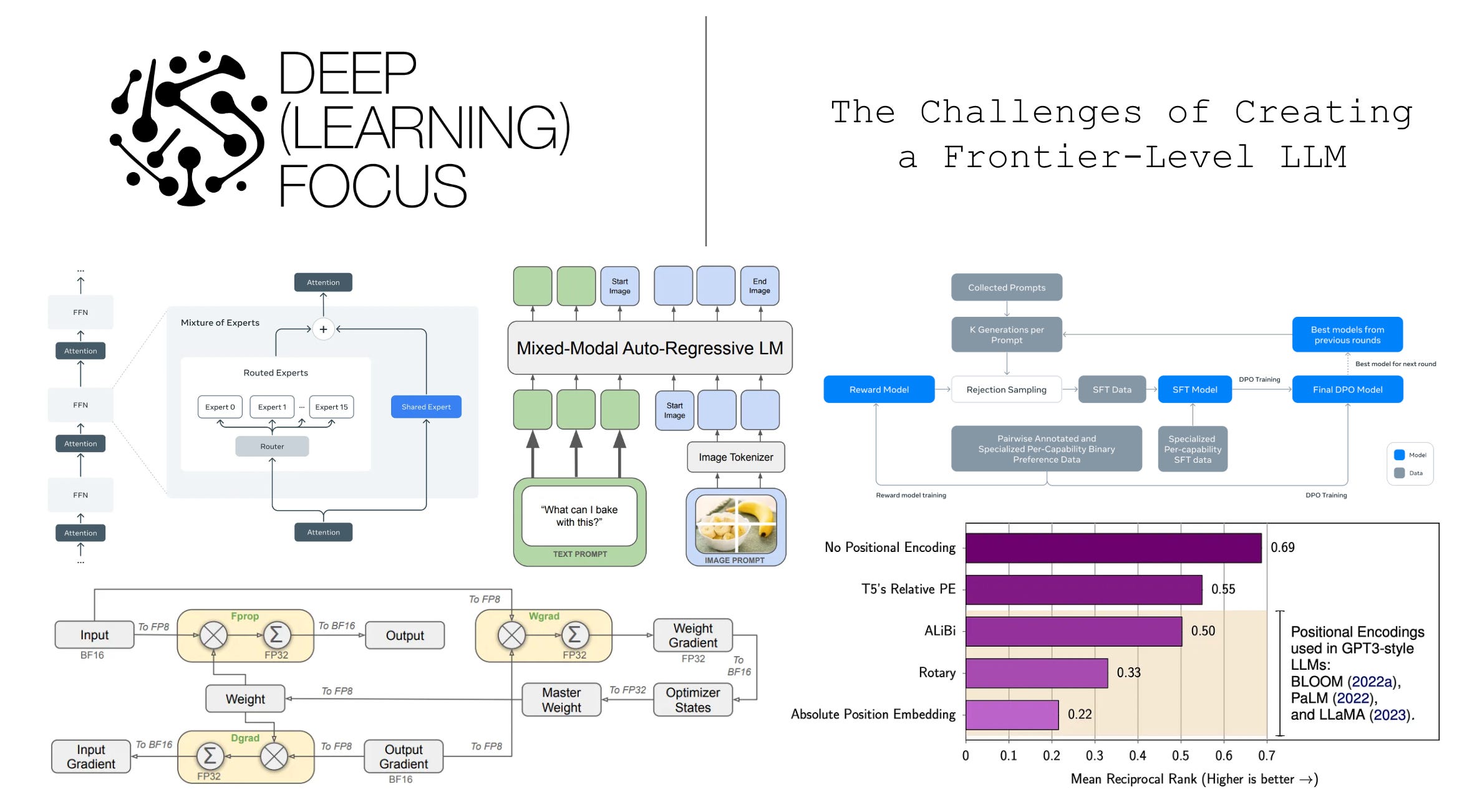
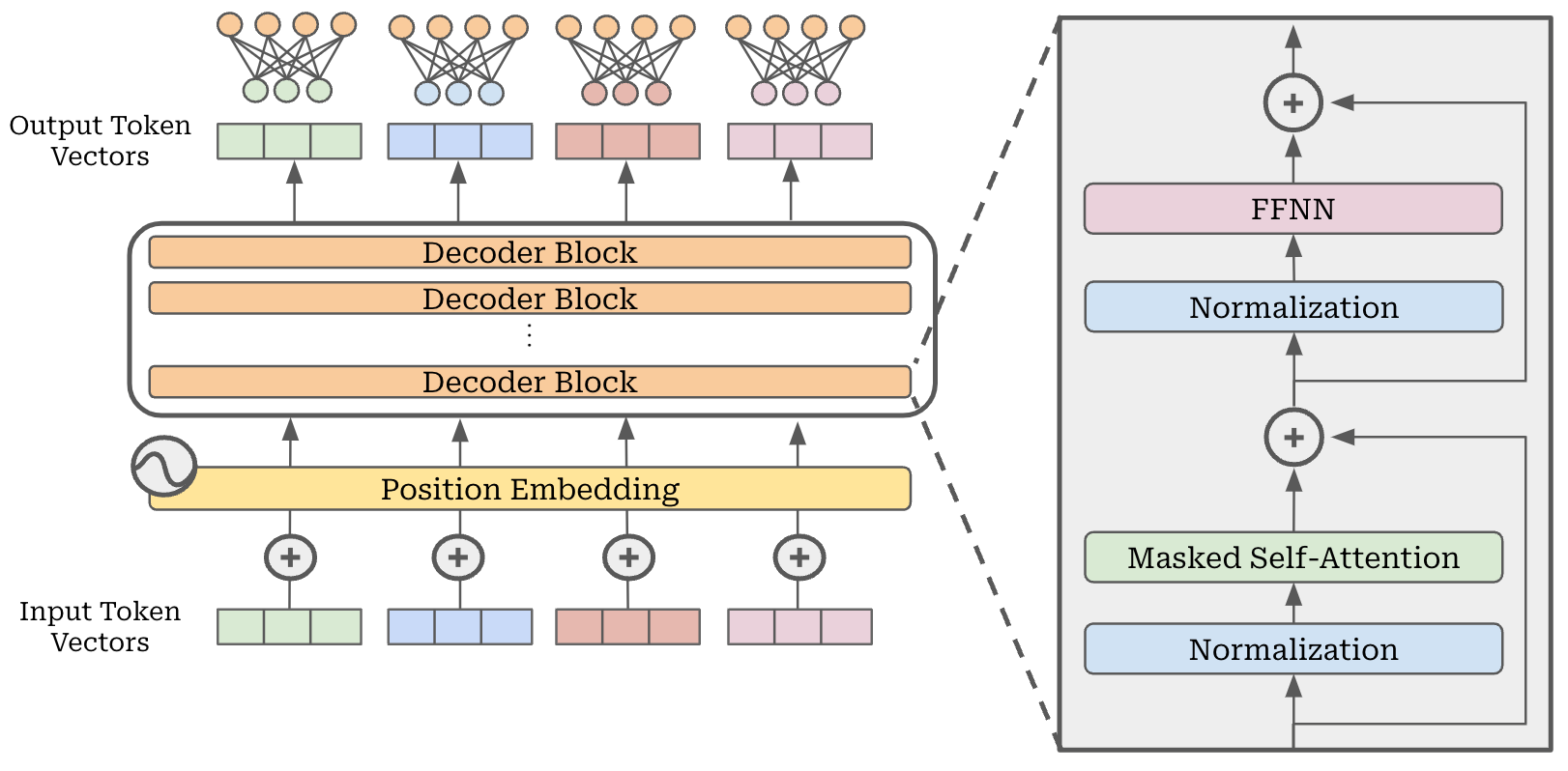
Instead of using a dense decoder-only transformer (depicted below), Llama 4 are the first of the Llama models to use a Mixture-of-Experts (MoE) architecture. Llama 3 avoided using an MoE for the purpose of stability and simplicity—larger MoE models introduce extra complexity to training and inference. With Llama 4, Meta falls in line with leading open (e.g., DeepSeek-v3 [4]) and proprietary models (e.g., GPT-4) that have successfully adopted the MoE architecture.

Put simply, dense models—though simple and effective—are difficult to scale. By using an MoE architecture, we can drastically improve the training (and inference) efficiency of very large models, thus enabling greater scale.

What is an MoE? Most readers will be familiar with the motivation of using an MoE—it is a modified version of the decoder-only transformer architecture that makes large models more compute efficient. Most of the key ideas behind MoEs were proposed in the three papers below, and we will overview these ideas here.

• The Sparsely-Gated Mixture-of-Experts Layer

• Switch Transformers

• Stable and Transferable Mixture-of-Experts (ST-MoE)

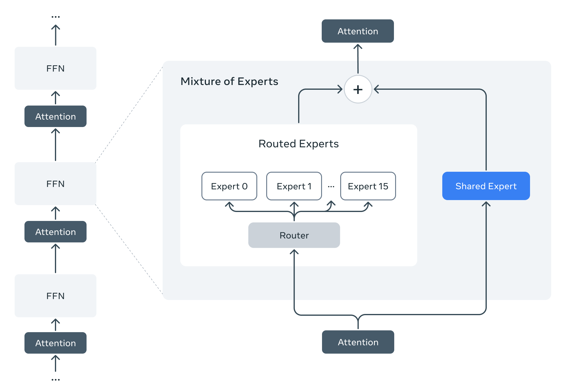
Compared to the decoder-only transformer, MoEs modify the feed-forward component of the transformer block. Instead of having a single feed-forward network in each block, we have several feed-forward networks, each with their own independent weights. We refer to each of these networks as an “expert”; see below.

To create an MoE architecture, we convert the transformer’s feed-forward layers into MoE—or expert—layers. Each expert in the MoE is identical in structure to the original, feed-forward network from that layer, and we usually convert only a subset of transformer layers into MoE layers; e.g., Llama 4 uses interleaved MoE layers where every other layer of the transformer becomes an expert layer.

“Our new Llama 4 models are our first models that use a MoE architecture… MoE architectures are more compute efficient for training and inference and, given a fixed training FLOPs budget, delivers higher quality compared to a dense model.” – from Llama 4 blog [1]

Routing mechanism. Obviously, making multiple copies of each feed-forward network in the transformer does not improve compute efficiency. To get an efficiency gain, we need to add sparsity. In other words, we don’t use every expert in each MoE layer. Instead, we select a subset of experts (e.g., one or two experts)—referred to as the “active” experts or parameters—to use for each token. This selection is done by passing each token vector through a linear layer that outputs a probability distribution over the set of experts; see below.

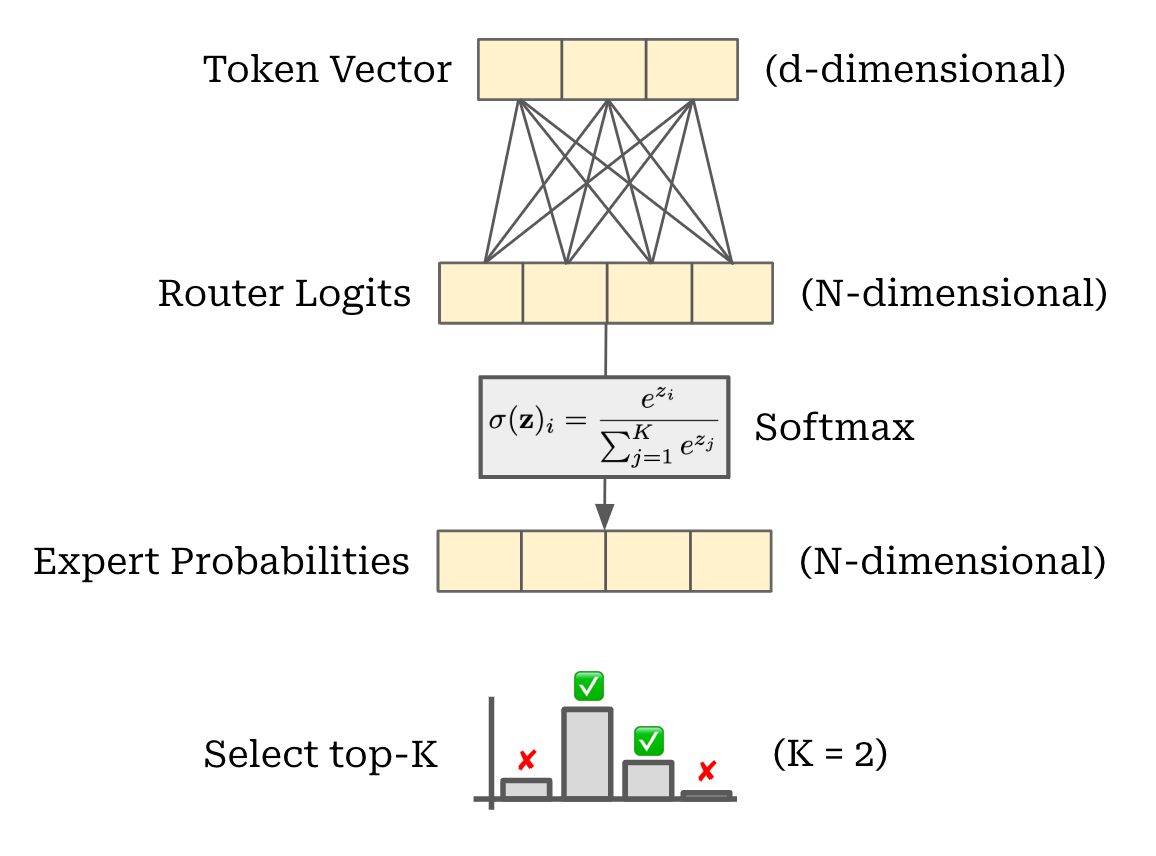
From here, we can process each token using only the experts that receive the highest probability. By doing this, we only use a portion of the model’s total parameters for each token—the number of active parameters is much smaller than the model’s total parameters. For this reason, we can train models with a large number of total parameters while incurring only a fraction of their total compute cost.

“The gating network tends to converge to a state where it always produces large weights for the same few experts. This imbalance is self-reinforcing, as the favored experts are trained more rapidly and thus are selected even more by the gating network.” – source

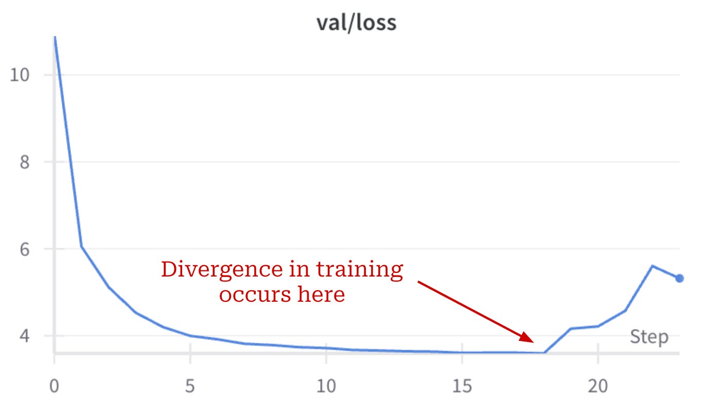
Load balancing and training stability. If we train an MoE similarly to a standard dense model, several issues are likely to occur. First, the model will quickly learn to route all tokens to a single expert—a phenomenon known as “routing collapse”. Additionally, MoEs are more likely to experience numerical instabilities during training, potentially leading to a divergence in the training loss; see below.

To avoid these issues and ensure that training is stable, most MoEs employ a load-balancing loss during training, which rewards the MoE for assigning equal probability to experts and routing tokens uniformly. Load-balancing losses modify the underlying training objective of the LLM by adding an extra loss term to the standard, next-token prediction loss; see below. As such, these auxiliary losses can impact the performance of the model, which has led some popular MoE-based LLMs (e.g., DeepSeek-v3) to avoid them altogether.

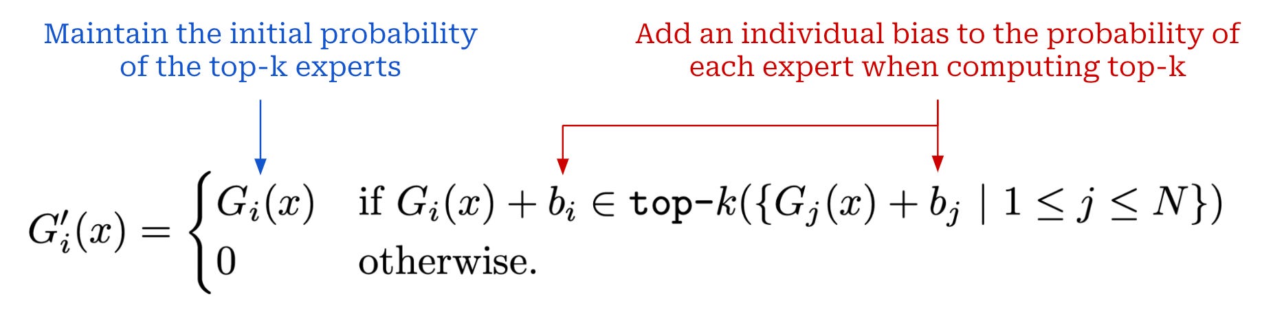
No statement is made in [1] as to the exact auxiliary losses used to train Llama 4 models (if any). To avoid training instability, we can use an auxiliary-loss-free load-balancing strategy similarly to DeepSeek-v3 and adopt a variety of extra tricks; e.g., better weight initialization or selective precision.

The primary takeaway we should glean from this information is the simple fact that MoEs—despite their many benefits—are much harder to train compared to standard dense models. This is a classic tradeoff between simplicity and performance! These architectures are more complex. Therefore, there are more factors to consider and many more issues that can occur during training. For more details on MoE architectures and training, check out the links below.

• Understanding MoE-based LLMs

• nanoMoE: Implementing an MoE-based LLM in PyTorch

Llama 4 architecture. Three flavors of Llama 4 models are presented in [1]:

• Scout: 109B total parameters, 17B active parameters, 16 experts per layer.

• Maverick: 400B total parameters, 17B active parameters, 128 experts per layer.

• Behemoth: 2T total parameters, 288B active parameters, 128 experts per layer.

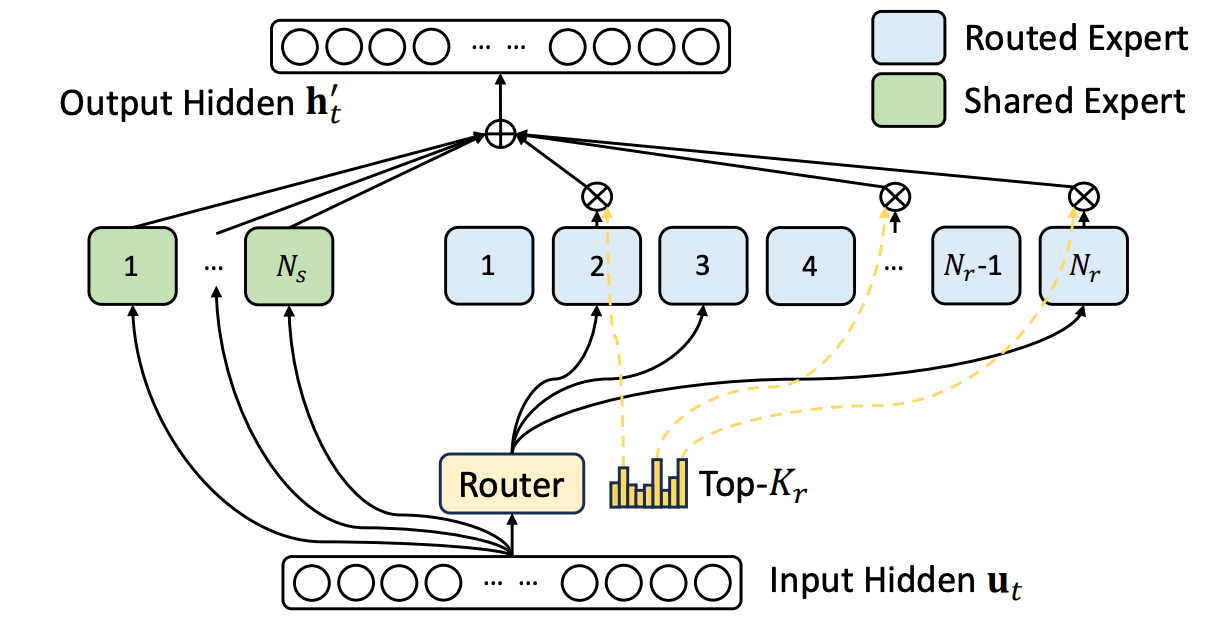
Both the Llama 4 Scout and Maverick models are released openly—under the Llama 4 community license agreement—in [1], while the Behemoth model was just previewed (i.e., not yet released). Similarly to DeepSeek-v3, Llama 4 models use both shared and routed experts. For example, Llama 4 Maverick has one shared expert—meaning that all tokens are passed to this expert with 100% probability—and selects one active routed expert per token using a routing mechanism; see below.

Relative to other popular MoEs, Llama 4 models have a very small number of active parameters. However, these architectural settings are not uncommon when compared to top industry labs:

• Scout optimizes for inference efficiency and is reminiscent of models like Gemini Flash or GPT-4o-mini.

• Maverick has an architecture that is relatively similar to DeepSeek-v3 (i.e., sparse model with a very large number of experts).

• Behemoth—the most powerful model in the suite—is a GPT-4-esque, multi-trillion parameter foundation model.

However, there are still differences between Llama 4 models and other popular LLMs. Only a single routed expert is selected per layer in Llama 4, whereas DeepSeek has multiple shared experts and eight active routed experts per layer (i.e., 37B active parameters and 671B total parameters). This smaller number of active parameters improves both the training and inference efficiency of Llama 4. In fact, Llama 4 models were reported to have used less compute during training relative to Llama 3 despite a drastic increase in data and model scale.

Fine-grained experts. One popular design choice made by several modern MoE-based LLMs (e.g., DeepSeek-v3 and DBRX) is the use of fine-grained experts. To use fine-grained experts, we just:

1. Increase the number of experts in each MoE layer.

2. Decrease the size (number of parameters) for each individual expert.

Usually, we also select a larger number of active experts in each layer to keep the number of active parameters (relatively) fixed in a fine-grained MoE model. We see both fine and coarse-grained experts used in the Llama 4 suite—the Scout model has 16 total experts, while Maverick has 128 total experts. Given that Maverick has 16× the number of experts but only 4× the number of total parameters compared to the smaller Scout model, it must be using fine-grained experts.

In contrast, both the Scout and Behemoth models use standard (coarse-grained) experts. There are a few different reasons that Meta may be making this choice. Generally, using fine-grained experts allows for more specialization among experts and can improve both performance and efficiency. However, fine-grained experts also introduce added complexity into the distributed training process.

Experts are typically distributed across multiple GPUs during training (i.e., expert parallelism); see above. When using coarse-grained experts, it is common for each GPU to store a single expert1. However, we can usually fit multiple fine-grained experts into the memory of a single GPU. Additionally, because we usually select a larger number of experts when using fine-grained experts, we could run into an issue where each token has to be routed to multiple different GPUs in the cluster, thus creating a drastic increase in communication costs between GPUs.

“We ensure that each token will be sent to at most 𝑀 nodes, which are selected according to the sum of the highest 𝐾 / 𝑀 affinity scores of the experts distributed on each node. Under this constraint, our MoE training framework can nearly achieve full computation-communication overlap.” – from DeepSeek-v3 paper [4]

As a result, we must adopt some strategy to limit communication costs and improve training efficiency. For example, DeepSeek-v3 uses the node-limited routing scheme described above, which restricts the number of devices to which a single token can be routed. We can avoid this extra complexity by not using fine-grained experts. However, training both fine-grained and coarse-grained expert models also provides more configurability and choices to model users.

Impact to open LLMs. MoEs do not use all of their parameters during inference, but we still have to fit the model’s parameters into GPU memory. As a result, MoE-based LLMs have a much higher memory footprint—and therefore require access to more and better GPUs—relative to dense models2. Llama 4 Scout “fits on a single H100 GPU (with Int4 quantization)”3, while Maverick needs “a single H100 host”. In other words, we cannot perform inference of the larger Maverick model using a single GPU—we have to perform distributed inference on a multi-GPU host.

With all of these considerations in mind, we may start to realize that the migration of Llama to an MoE architecture is a double-edged sword:

• The Llama project takes a step towards parity with the most powerful (proprietary) LLMs and unlocks potential for creating better models.

• The barrier to entry for using Llama models is increased.

This dilemma has significant implications for open LLM research. Increasing the barrier to entry for open LLMs has significant side effects and will hinder the ability of those without significant GPU resources to conduct meaningful research. The open LLM community cannot continue to thrive its contributors are slowly priced out of doing research as models continue to advance.

“The model that becomes the open standard doesn’t need to be the best overall model, but rather a family of models in many shapes and sizes that is solid in many different deployment settings… memory-intensive models like sparse MoEs price out more participants in the open community.” – Nathan Lambert

To avoid this negative aspect of MoE architectures, we can distill larger MoE models into smaller dense models, providing a suite of more user-friendly LLMs that still perform well. This approach was adopted and popularized by DeepSeek-R1 [5]4, a 671B parameter MoE-based reasoning model that was distilled into several dense LLMs with sizes ranging from 1.5B to 70B parameters. One of the key findings from [5] is the fact that distillation is most effective when a very large and powerful model is used as a teacher. As we will see later in the overview, distillation from Llama 4 models is already being heavily explored.

Native Multi-Modality and Early Fusion

Multi-modal Llama models have been released in the past. The original Llama 3 publication [2] included preliminary experiments with multi-modality, which were later productionized with the release of Llama 3.2 Vision. Key details of multi-modal Llama 3 models are outlined within the overview linked below. Similarly to prior model generations, Llama 4 models support visual inputs—both images and videos. However, as we will see in this section, Llama 4 takes a drastically different approach to multi-modality.

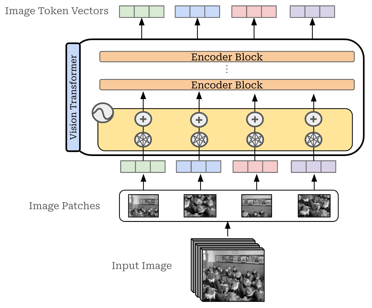
Multi-modal architectures. Multi-modal LLMs have two primary components: an LLM backbone and a vision encoder. The LLM backbone is just a standard decoder-only transformer, while the vision encoder is usually a CLIP or ViT model that converts an image into a set of corresponding embeddings; see below.

Given these two components, a vision LLM (or vLLM for short) must learn how to properly fuse both visual and textual information. In other words, the LLM must somehow i) ingest the image embeddings and ii) use these embeddings as added context for generating text. There are two primary model architectures that can be used for this purpose (depicted below):

1. Unified embedding: concatenates both image and text tokens at the input layer to form a single input sequence that is processed by the LLM5.

2. Cross-modality attention: passes only text tokens as input to the LLM and fuses visual information into the model via additional cross-attention layers.

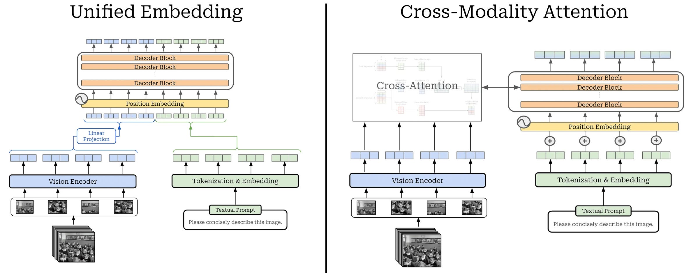
These architectures both have their benefits. For example, cross-modality attention tends to be more efficient because we do not pass image embeddings through the entire LLM backbone. However, the unified embedding approach has the potential to yield better performance for the same exact reason!

Multi-modal training. Given that vLLMs generate text as output, we still train them using next token prediction. Beyond the training objective, however, there are a few different choices of training strategies for these types of models:

1. Native multi-modality: train the vLLM from scratch using multi-modal data from the beginning.

2. Compositional multi-modality: begin by training a separate LLM backbone and vision encoder, then perform extra training to fuse them together.

Objectively speaking, native multi-modality introduces extra complexity into the training process (e.g., imbalances between modalities). Assuming that we can avoid these pitfalls, however, natively multi-modal training has massive potential—it expands the scope and volume of data to which the model can be exposed. For this reason, many top labs—most notably Google and OpenAI—have adopted this approach, which was likely a motivating factor for the design of Llama 4.

“Llama 4 models are designed with native multimodality, incorporating early fusion to seamlessly integrate text and vision tokens into a unified model backbone. Early fusion is a major step forward, since it enables us to jointly pre-train the model with large amounts of unlabeled text, image, and video data.” – from Llama 4 blog [1]

Prior Llama variants (e.g., Llama 3.2 Vision) use a cross-modality attention architecture and are trained with a compositional approach. In contrast, Llama 4 models are natively multi-modal and are pretrained from scratch using text, image and video data. Migrating to native multi-modality allows Llama 4 models to draw upon multiple modalities of data when constructing their massive 30T token pretraining dataset—more than 2× larger than that of Llama 3.

Early fusion. As indicated in the above quote, Llama 4 also adopts a unified embedding architecture instead of the cross-modality attention architecture that is used by Llama 3. In [1], the term “early fusion”, meaning that images and text are combined at the input-level of the LLM, is used to describe the architecture of Llama 4 models. Alternatively, “late fusion” architectures (e.g., cross-modality attention) combine image and text data in a later layer of the LLM.

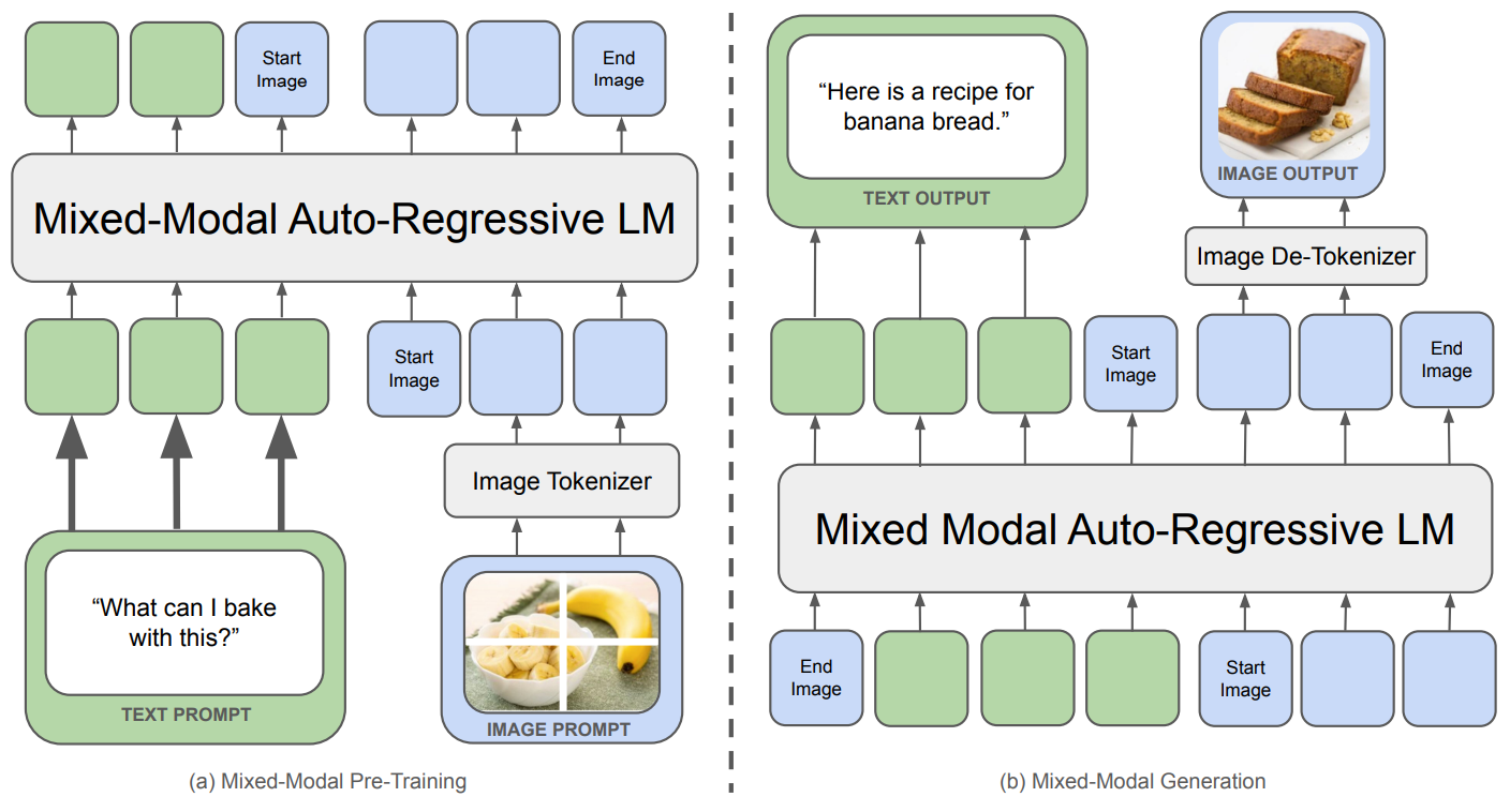
Although authors do not provide many details on the architecture of Llama 4 in [1], we can look at Chameleon [6]—a recent publication from Meta on the topic of native multi-modality and early fusion—for hints on what might be happening in Llama 4. As shown above, the Chameleon architecture passes interleaved image and text tokens as a single sequence to a unified LLM backbone. This model is trained using a natively multi-modal approach and is even capable of generating images as output. Although no image generation capabilities are presented for Llama 4 in [1], we might expect such a capability in the near future based on Llama 4’s use of a Chameleon-style early fusion architecture and the recent success of OpenAI in image generation with natively multi-modal models.

“This early-fusion approach, where all modalities are projected into a shared representational space from the start, allows for seamless reasoning and generation across modalities. However, it also presents significant technical challenges, particularly in terms of optimization stability and scaling.” – from [6]

In [6], authors mention that they experience a variety of unique difficulties when training Chameleon largely due to the model’s native multi-modality. Namely, Chameleon experiences more frequent training instabilities and is harder to scale compared to a standard text-based LLM. To get around these issues, a few notable modifications are made to the underlying transformer architecture:

• Layer norm is applied to the query and key vectors during attention6.

• An additional dropout module is added after each attention and feed-forward layer in the transformer.

• The position of layer norm in the transformer block is modified (i.e., a post-norm structure is adopted instead of the more standard pre-norm [8]).

The difficulties outlined in [6] clearly demonstrate the technical complexity of natively multi-modal training. Although Llama 4 is not confirmed to use any of the architectural tricks from Chameleon, these lessons are universally useful for any model trained using a natively multi-modal approach.

The vision encoder. Although the Chameleon architecture largely matches the structure of the unified embedding model described above, the attentive reader may notice that Chameleon has no image encoder! Instead, we directly quantize images into discrete token embeddings, as described in this paper.

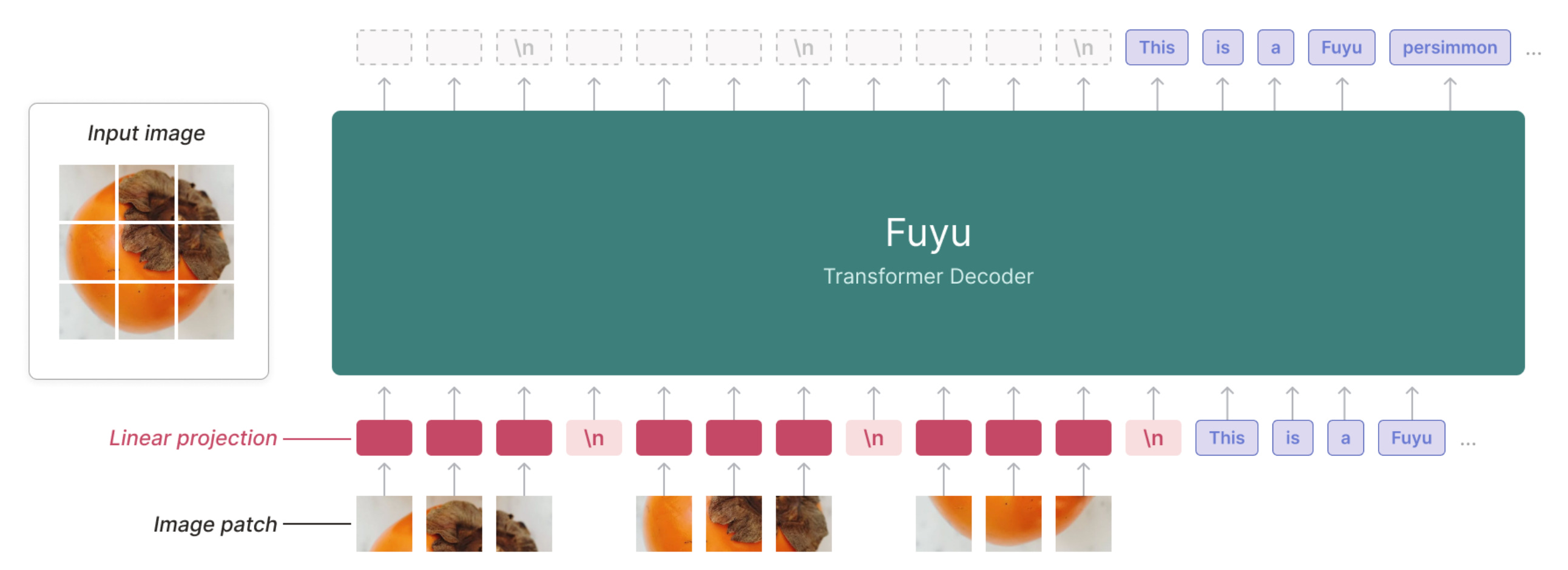
Chameleon is not the first model to forgo image encoders and directly pass image info as input to an LLM. Fuyu [7] breaks images into patches—like a standard ViT—and linearly projects these patches to make them the same size as a text token vector. Then, the LLM can directly ingest these image patch embeddings as input. The main motivation for this approach is the fact that relevant information from the image may be lost when we pass that image through a vision encoder.

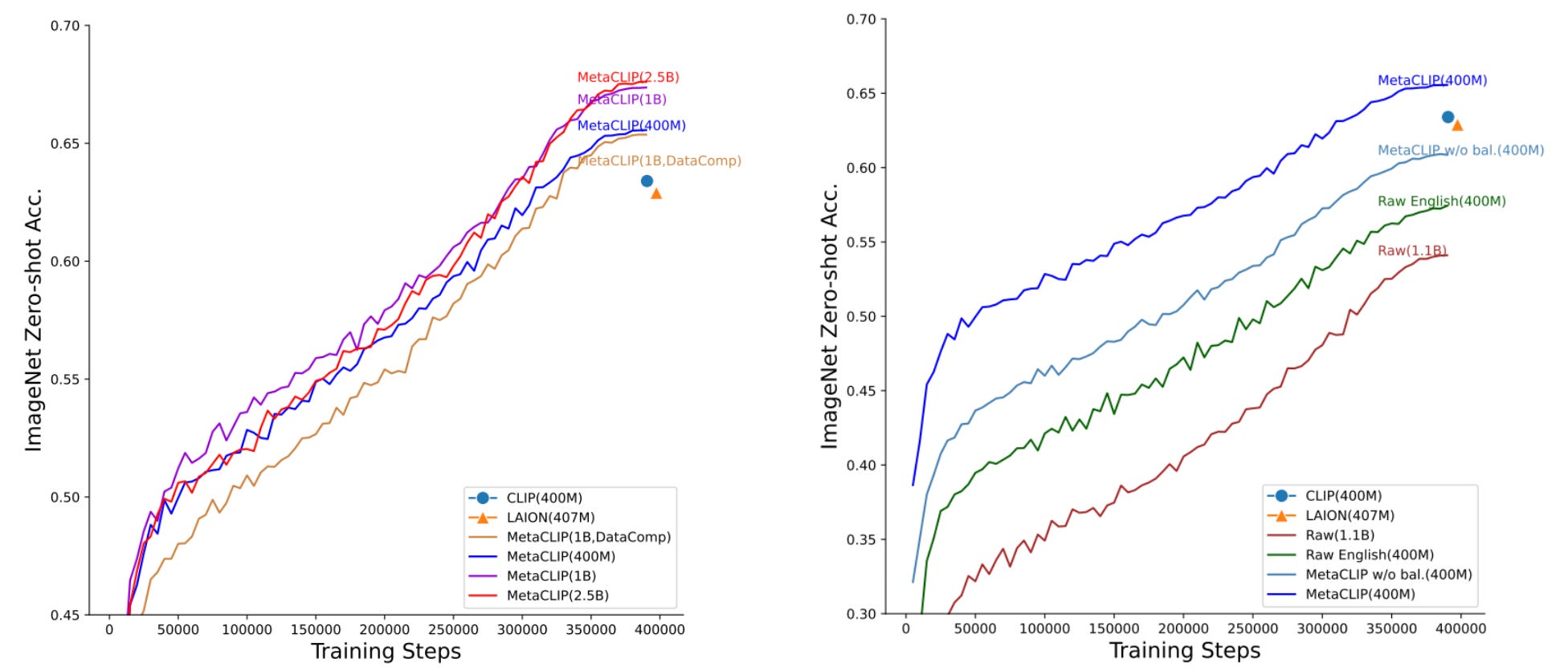
Unlike Chameleon, authors confirm in [1] that Llama 4 uses a vision encoder that is based upon MetaCLIP [9]—an open replication of CLIP that emphasizes training data transparency. Llama 3 uses the same architecture for its vision encoder. However, the Llama 4 vision encoder is trained in conjunction with an LLM to both i) improve the quality of its embeddings and ii) better align the visual embeddings with textual embeddings from the LLM.

“We also improved the vision encoder in Llama 4. This is based on MetaCLIP but trained separately in conjunction with a frozen Llama model to better adapt the encoder to the LLM.” – from Llama 4 blog [1]

10M Token Context Window

Long context understanding is important, both for solving tasks that naturally require long context (e.g., multi-document summarization) and reasoning-based use cases. Many top labs have released models with massive context windows to enable more long context applications. The release of Llama 4 follows the trend towards longer context and tries to set a new state-of-the-art in this area. As we will learn, however, enabling long context is highly complex and typically requires the (correct) integration of numerous interrelated techniques into the LLM.

10M token context. Extending upon Llama 3’s context length of 128K tokens, Llama 4 Scout has an industry-leading context length of 10M tokens. The model is pretrained with a context length of 256K tokens, but the 10M token context is made possible via a variety of tricks involving modified position embeddings, scaled softmax, and long-context focused training procedures. Let’s dive deeper into the details of these techniques to understand exactly how they work.

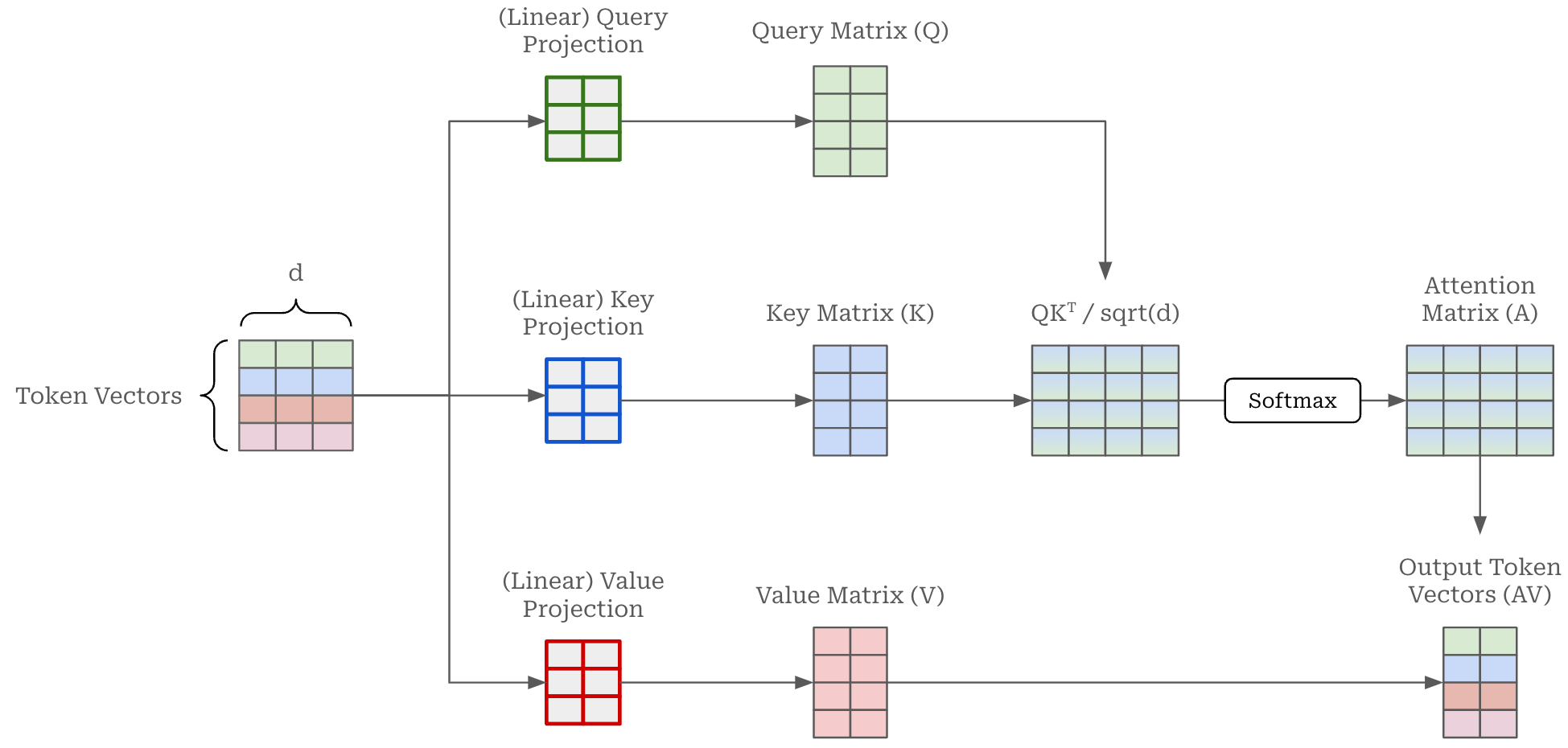
Position embeddings help the transformer to understand the order of tokens in a sequence; e.g., which token comes first, second, third and so on. Explicit position information is necessary because self-attention does not naturally consider the ordering of a sequence. Rather, all tokens in the sequence are considered simultaneously—agnostic of position—as we compute attention scores between them; see above. By using position embeddings, we can directly inject position information into the embedding of each token, allowing self-attention to use this information and learn patterns in the ordering of tokens. Many position encoding schemes exist, such as standard Absolute Position Embeddings (APE), Rotary Position Embeddings (RopE) [11], Attention with Linear Biases (ALiBi), and more.

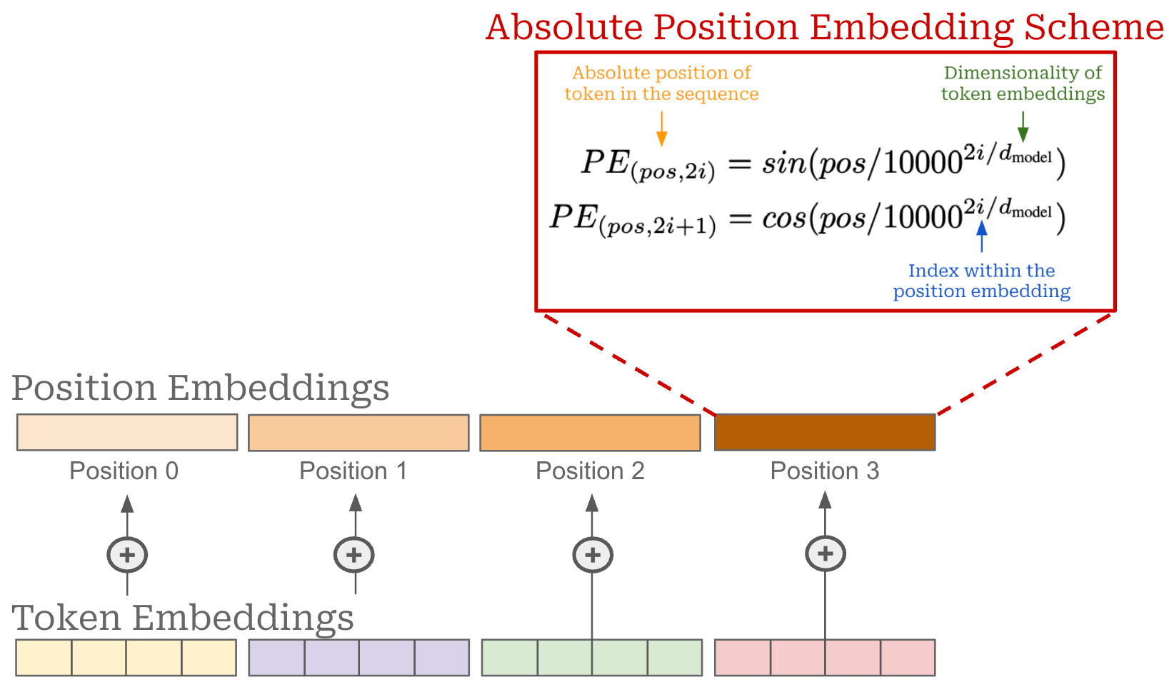
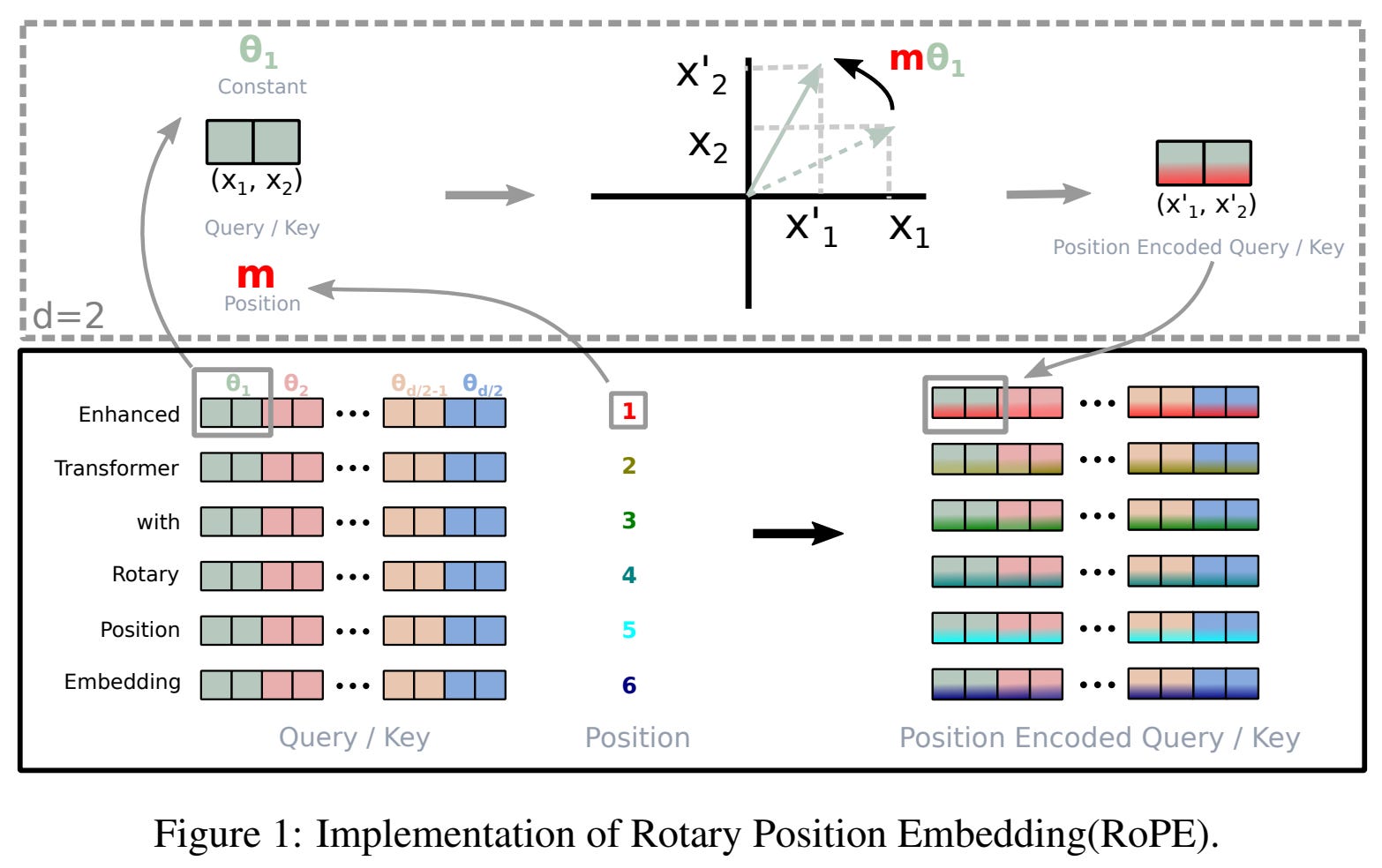
RoPE explained. The original transformer architecture uses an absolute position embedding scheme that adds a fixed position embedding to each token vector at the model’s input layer based upon the token’s absolute position in the sequence; see above. Today, LLMs more frequently use relative position embeddings that consider distances between tokens instead of absolute position. By using relative position embeddings, we can achieve better performance7 and make the attention mechanism more generalizable to sequences of different lengths. The most commonly-used position encoding scheme for LLMs is RoPE [11] (depicted below), which is used by both the Llama 3 [2] and Llama 4 [1].

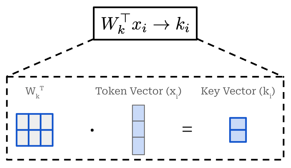
RoPE is a hybrid of absolute and relative position embeddings that operates by modifying the query and key vectors in self-attention. Unlike absolute position embeddings, RoPE acts upon every transformer layer—not just the input layer. In the standard transformer architecture, we produce key and query vectors by linearly projecting the sequence of token vectors for a given layer. For a single token in the input sequence, we can formulate this operation as shown below, where we linearly project a single token embedding. The figure below displays the creation of a key vector, but we follow the same exact approach—with a different weight matrix—to produce query and value vectors too.

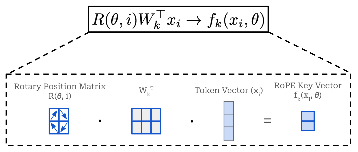
RoPE incorporates position information into the creation of key and query vectors by multiplying the weight matrix used in the above operation by a unique rotation matrix. Here, this rotation matrix is computed based upon the absolute position of a token in the sequence—the amount that a given vector is rotated depends upon its position in the sequence. This modified operation is shown below, where we again depict the creation of key vectors. The same strategy is applied to the creation of query vectors, but we do not modify the creation of value vectors.

Here, θ is a vector called the rotational (or frequency) basis. We have a function R that takes the rotational basis θ and the position of the token in the sequence i as input and produces a rotation matrix as output. The rotation matrix is a block-diagonal matrix that is constructed as shown in the equation below.

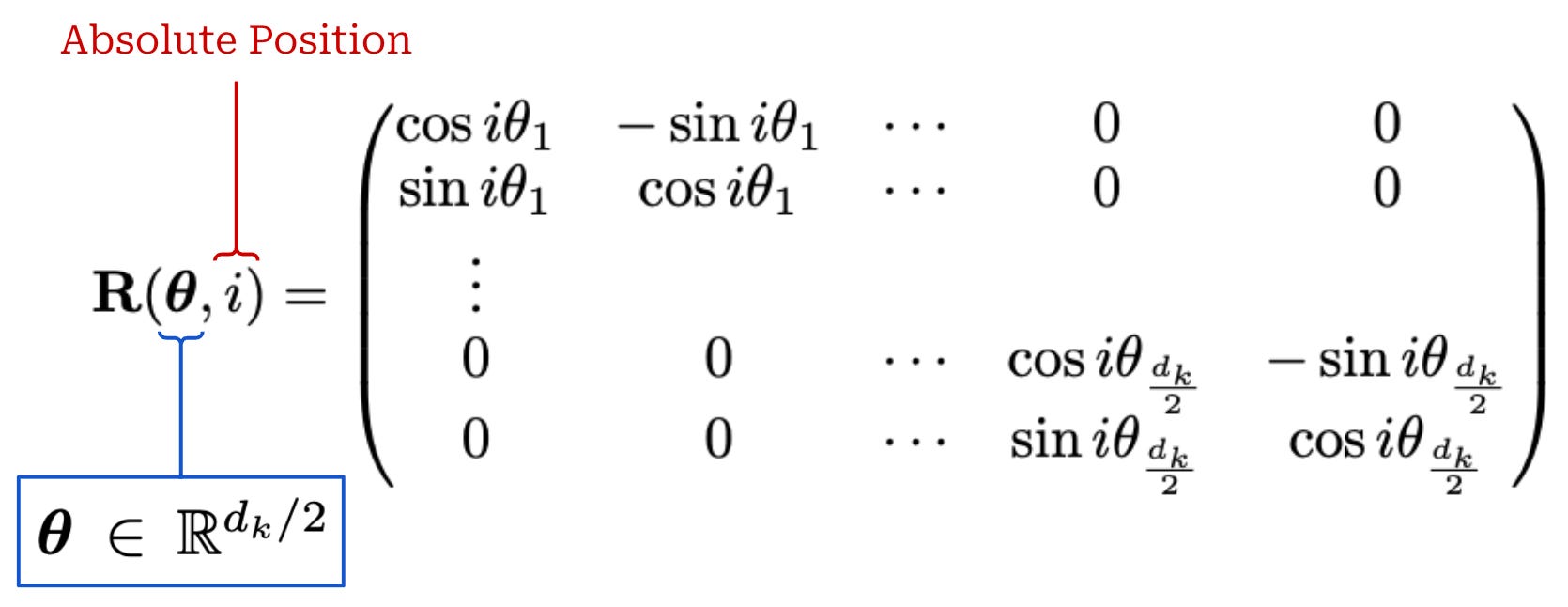
This matrix is block diagonal and each block in the matrix is a 2 × 2 rotation matrix. Each of these blocks rotates a pair of two dimensions within the output key (or query) embedding. As a result, each pair of dimensions in the resulting embedding is rotated based upon both the absolute position of the token in the sequence i and the entry of the rotational basis θ corresponding to that pair of dimensions. We apply this rotation matrix when producing both the key and query vectors for self-attention in every transformer layer. These modifications yield the attention operation shown below, where every key and query vector is rotated according to their absolute position in the sequence.

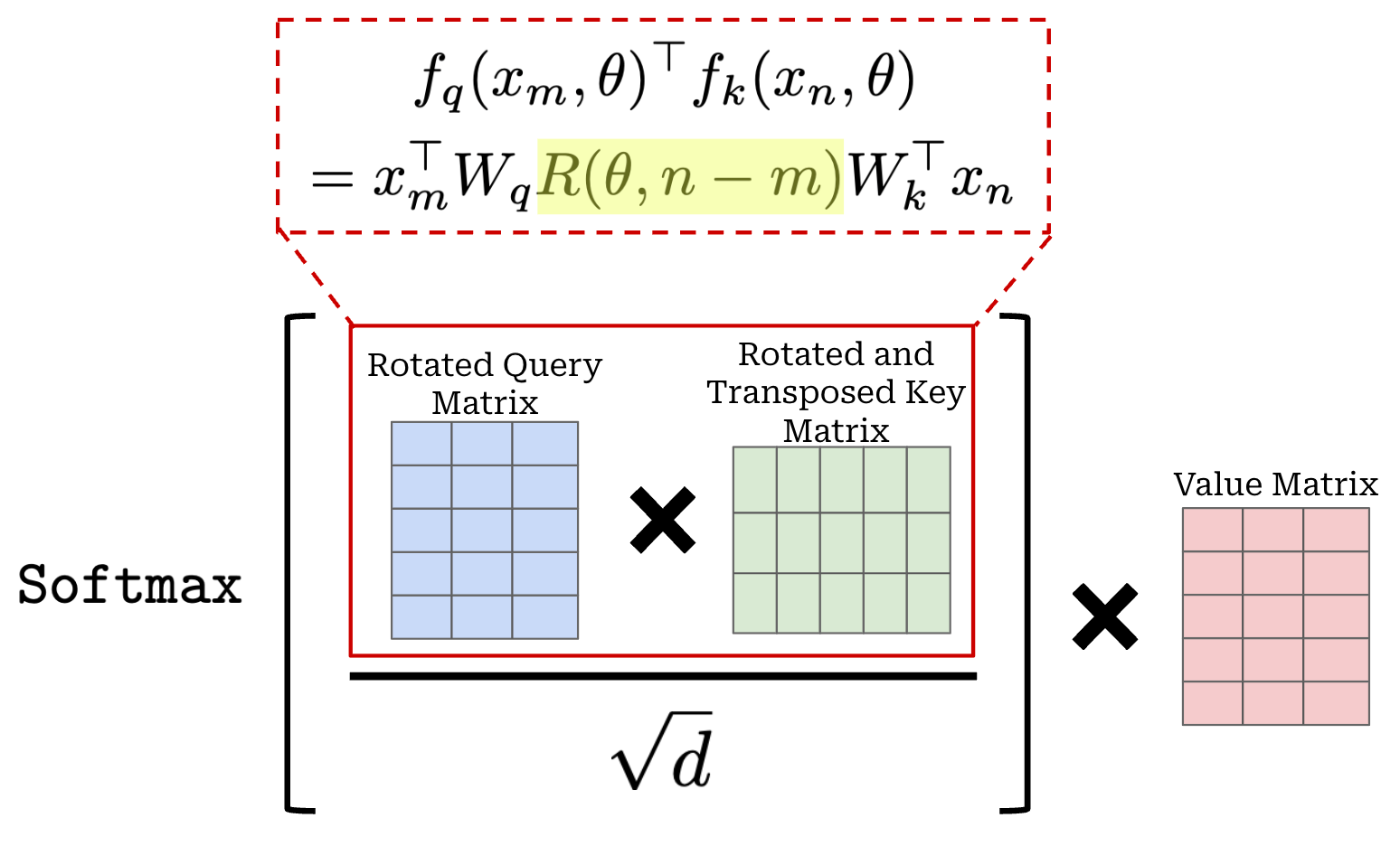
When we take this standard outer product between the rotated keys and queries, however, something interesting happens. The two rotation matrices—used to rotate the keys and queries, respectively—combine to form a single rotation matrix R(θ, n - m). In other words, the combination of rotating both the key and query vectors in self-attention captures the relative distance between tokens in the sequence. This is the crux of RoPE! Although we might struggle to understand the purpose of these rotation matrices at first, we now see that they inject the relative position of each token pair directly into the self-attention mechanism!

Length generalization. If we provide a sequence to an LLM that is much longer than the sequences upon which the model was trained, the performance of the model will drastically deteriorate. Position embeddings play a key role in an LLM’s ability to generalize to longer context lengths. Ideally, we want to use a position encoding scheme that allows the model to generalize more easily to context lengths that go beyond what is seen during training!

“Length generalization, the ability to generalize from small training context sizes to larger ones, is a critical challenge in the development of Transformer-based language models. Positional encoding has been identified as a major factor influencing length generalization.” – from [12]

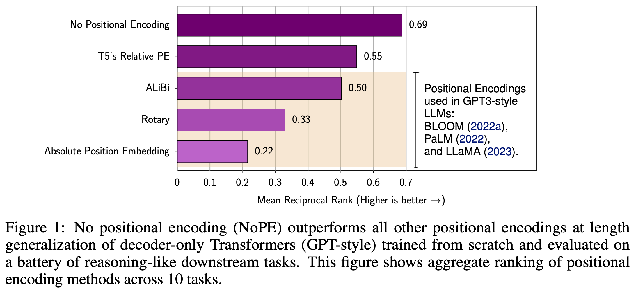
Recently, researchers showed that the most common position encoding schemes for LLM’s—including RoPE—fail to generalize well to long context lengths [12]; see below. Even though RoPE is generally considered to be a relative position encoding scheme, it performs similarly to absolute position encodings when generalizing to long context lengths. However, the No Positional Embedding (NoPE) scheme proposed in [12], which simply removes position embeddings from the model, is surprisingly capable of generalizing to longer contexts.

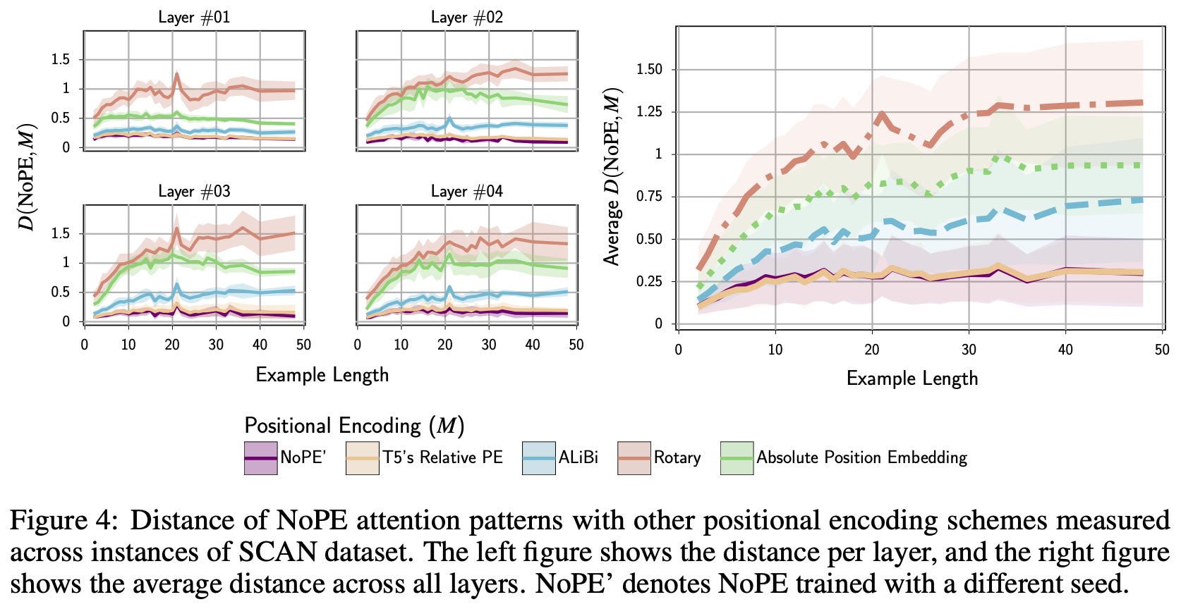
The fact that NoPE works well is surprising, but empirical (and theoretical) analysis in [12] reveals that transformers can represent both relative and absolute position encodings without using explicit position embeddings. Practically, the attention patterns learned by NoPE are shown to resemble relative position encodings in [12]; see above. Drawing upon these results, Llama 4 models interleave standard transformer layers that use RoPE with layers using NoPE. This approach, called interleaved RoPE (iRoPE), improves long context abilities.

“A key innovation in the Llama 4 architecture is the use of interleaved attention layers without positional embeddings. Additionally, we employ inference time temperature scaling of attention to enhance length generalization.” – from Llama 4 blog [1]

Temperature scaling. Every transformer layer has a softmax transformation within its attention mechanism. Softmax is computed for element i of an N-dimensional vector as follows:

The denominator of this expression—the sum of raw attention scores for all pairs of tokens in the sequence—will become larger with increasing context length, but the numerator is decoupled from the context length and fixed in magnitude. These two facts create an interesting phenomenon in attention scores for long contexts: attention scores get smaller as the context length grows larger. To mitigate this issue, authors in [13] propose Scalable-Softmax, which is formulated as follows:

Similarly to standard softmax, Scalable-Softmax is just a function that converts a vector of values into a valid probability distribution. However, this variant of the softmax introduces two new and important factors:

• s: a scaling parameter that can be tuned to change the function’s shape.

• N: the length of the input vector.

By including the length of the input vector in Scalable-Softmax, we can balance the scale of the numerator and denominator, prevent long context attention scores from decaying and improve long context capabilities; see below.

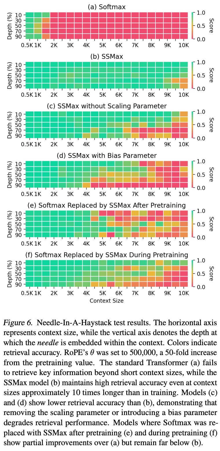
As mentioned in [1], Llama 4 models adopt a similar approach that scales the temperature of the softmax function at inference time to avoid attention scores from decaying at very large context lengths. Lowering the softmax temperature makes the resulting distribution more pointed, while increasing the temperature makes the distribution more uniform. We can simply lower the temperature of softmax at long context lengths to balance attention scores. Such inference-time tricks are useful, but they also complicate the inference process of Llama 4, thus increasing the likelihood of detrimental bugs and implementation differences.

Context extension. Finally, in addition to the strategies outlined so far, we need to train the LLM to support long context. Usually, we do not just pretrain the LLM with long context. Such an approach is sub-optimal because the memory requirements of training on long sequences are very high. Instead, we can train the model in two stages:

1. Standard pretraining with lower context length.

2. Finetuning on a long context dataset, also known as “context extension”.

For example, Llama 4 Scout is pretrained with a 256K context length prior to having its context extended during a later stage of training.

“We continued training the model in [mid-training] to improve core capabilities with new training recipes including long context extension using specialized datasets. This enabled us to enhance model quality while also unlocking best-in-class 10M input context length for Llama 4 Scout.” – from Llama 4 blog [1]

By dedicating a specific finetuning stage to context extension, we can limit the amount of training performed with ultra-long sequences. In most cases, the training data used for context extension is synthetic—either created with heuristics or an LLM—due to the difficulty of collecting real long-context data. As we will see, the quality of the synthetic data used for context extension can drastically impact the model’s capabilities. This data must accurately resemble and capture the types of tasks that the model will solve in practice. As we will see, the long context abilities of Llama 4 models break down in practice, possibly due to this issue.

In [1], authors do not mention the exact methods used for extending the context of Llama 4. However, we can overview some commonly-used techniques in the literature to provide inspiration for the context extension techniques that Llama 4 likely used. As described perfectly in the above video, there are two main categories of approaches used for extending the context of an LLM:

• Position Interpolation: these techniques adjust the frequency basis of RoPE8 such that larger positions still fit within the model’s “known” context length; e.g., Position Interpolation, NTK-RoPE, YaRN, and CLEX.

• Approximate Attention: these techniques modify the structure of attention to only consider certain groups of tokens (e.g., based on a blocks, landmarks or a sliding window) when computing attention scores.

An extensive analysis of these approaches is provided in [14], where we see that position interpolation-style methods tend to perform the best. In particular, NTK-RoPE achieves very impressive performance due to its ability to dynamically adjust frequencies in RoPE so that the frequency of nearby tokens is not changed too much. These techniques are very commonly used for training LLMs. As a concrete example, see page four of the Qwen-2.5 report where authors describe increasing the base frequency of RoPE before performing long context training.

Training Llama 4

In addition to its completely revised architecture, Llama 4 uses a new training pipeline that makes significant modifications to both pre and post-training. Again, many of these changes introduce extra complexity for the purpose of better performance and are inspired by techniques that have been successfully adopted within frontier-level research labs. Interestingly, the training process for the smaller Llama 4 Maverick and Scout models also heavily leverages knowledge distillation from the much larger Behemoth model.

Pretraining

Significantly tweaking the pretraining process for an LLM is both risky and rare given that i) pretraining is very expensive and ii) techniques for pretraining and scaling are heavily studied and (relatively) solidified. However, the native multi-modality and MoE-based architecture of Llama 4 warrant some changes to the pretraining process that we will quickly overview in this section.

Native multi-modality. As mentioned previously, Llama 4 models are pretrained over a massive 30T token dataset comprised of text, images and videos. However, this dataset is not just multi-modal, it’s also highly multilingual and contains data from 200 languages. Over 100 of these languages have at least 1B training tokens associated with them, providing a 10× increase in multilingual data relative to Llama 3. This multilingual emphasis is not surprising given Meta’s prior investments into machine translation research, most notably their No Language Left Behind (NLLB) model that also supports 200 languages.

“In the final stages of pre-training, we train on long sequences to support context windows of up to 128K tokens. We do not train on long sequences earlier because the compute in self-attention layers grows quadratically in the sequence length.” – from Llama 3 paper [2]

Llama 4 models are pretrained using a context length of 256K tokens, which is quite large compared to prior models. For example, Llama 3 is originally pretrained with a context length of 8K, which is later increased to 128K via a six-stage context extension process. This extended context length speaks to the efficiency of the pretraining process with Llama 4’s new MoE architecture and is needed for multi-modal pretraining. Namely, Llama 4 receives up to 48 images—either standalone images or still frames from a video—in its input sequence during pretraining and provides good results with up to eight images during testing.

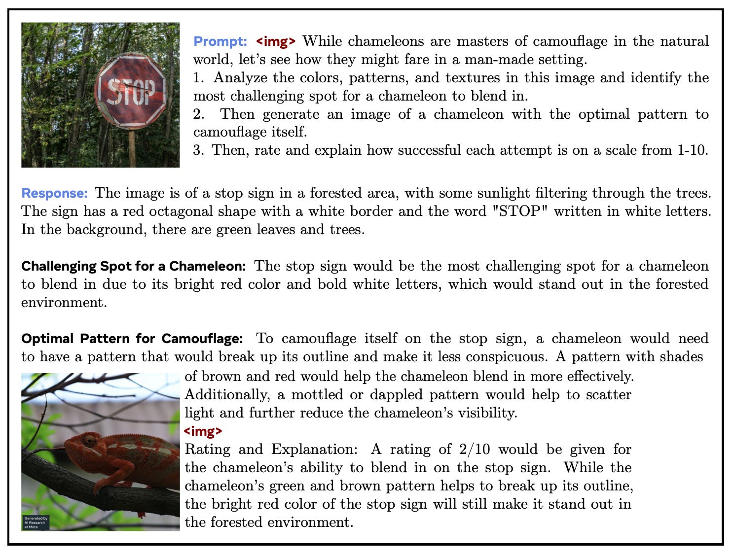
Given that Llama 4 uses a (Chameleon-style) unified embedding architecture, images and video stills can be arbitrarily interleaved within the model’s input sequence; see above. Here, visual tokens are just another token in the model’s input sequence and are treated similarly to a standard text token. Unlike Llama 3, the Llama 4 blog [1] does not explicitly mention the use of a Perceiver Resampler for ingesting video data. Instead, it seems—based on wording in the blog post—that the model might just ingest still video frames and learn temporal patterns from the position of each token within the input.

“Compared with the BF16 baseline, the relative loss error of our FP8-training model remains consistently below 0.25%, a level well within the acceptable range of training randomness.” – from [4]

Low precision training. Authors in [1] mention that Llama 4 models are trained using FP8 precision. DeepSeek-v3 [4] was the first open model to successfully use FP8 precision for large-scale pretraining. Mixed precision training is common, but FP8 is an aggressive precision setting—most training is performed with higher precision like bfloat16. Plus, MoEs are especially sensitive to mixed precision training due to their increased likelihood of training instability.

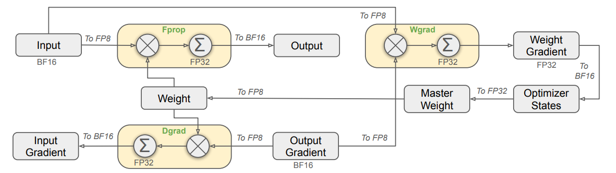
Few details are provided on the FP8 scheme used for training Llama 4, but the implementation is likely to resemble that of DeepSeek-v3; see above. The main issue with FP8 training is the presence of outliers within the activations, weights and gradients of an LLM—truncating the precision of large numbers leads to round-off errors that create instabilities during training. To avoid this issue, DeepSeek-v3 proposes a novel FP8 quantization scheme that performs fine-grained quantization of 1D tiles or 2D blocks of values within the model. By performing quantization over finer-grained groups, we minimize round-off errors.

Curriculum learning. Finally, Llama 4 is also pretrained in multiple stages, including both the standard pretraining phase and an additional training phase—referred to as “mid-training” in [1]—with a different data mixture that emphasizes key domains and specific model capabilities (e.g., long context understanding). This strategy of annealing the mixture of data being used toward the end of pretraining is common for LLMs. For example, Llama 3 uses a similar strategy with a high-quality annealing dataset (see page 56 in the paper) and entire papers have even been published on exactly this topic [10]!

Post-Training

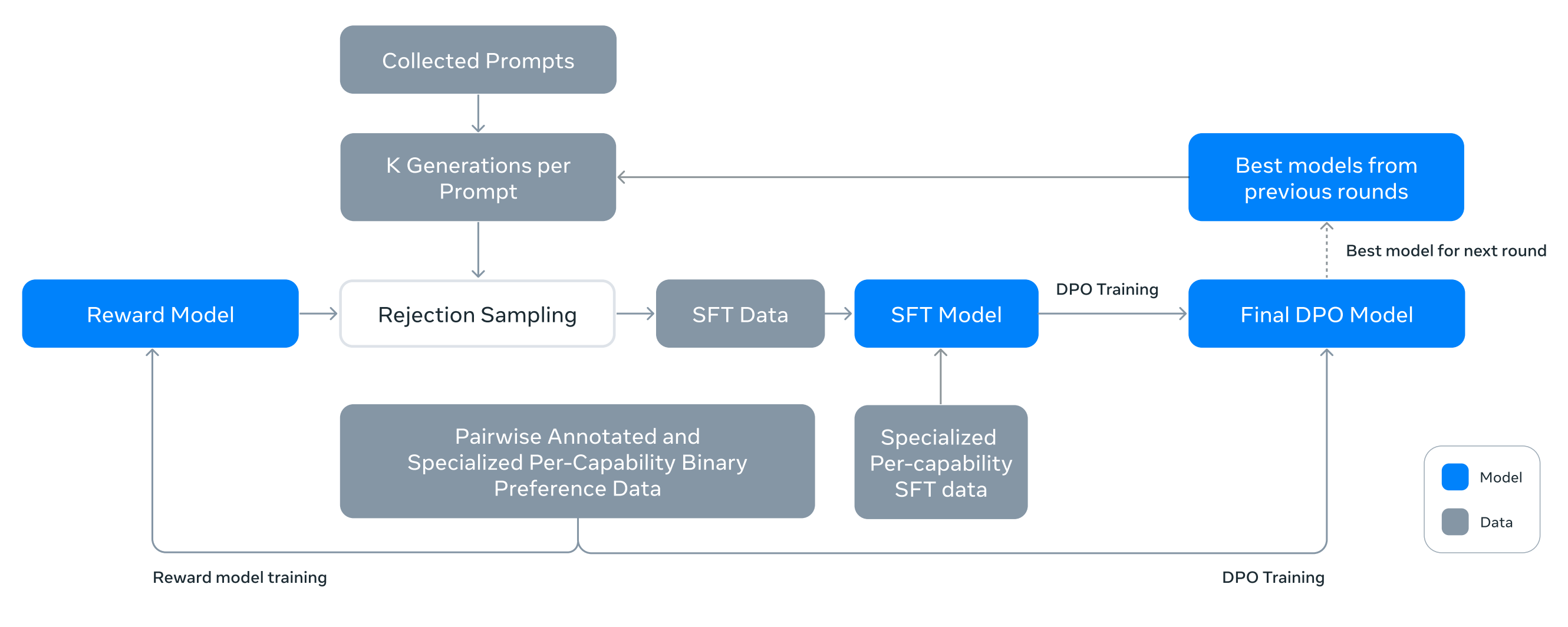
One of the most fascinating aspects of Llama 3 is the simplicity of its post-training pipeline, which includes several rounds of supervised finetuning (SFT) and direct preference optimization (DPO) [18]; see above. Given that DPO does not require the training of a separate reward model like PPO-based RLHF, this strategy is more user friendly in terms of the required GPU resources. However, we see with Llama 4 that such a basic alignment strategy comes at the cost of model performance. Post-training is one of the fastest-moving domains of LLM research, and a more sophisticated approach is needed to match top models. For a more general overview of LLM post-training, see the video below.

Post-training for Llama 4. Post-training for Llama 4 has three key stages:

1. Lightweight SFT: supervised training over a small (and highly-curated) set of completions for difficult prompts.

2. Online RL: large-scale RL training focused on improving model capabilities in several areas (e.g., multi-modality, reasoning, conversation and more).

3. Lightweight DPO: a short additional training phase used to fix minor issues and corner cases in model response quality.

Put simply, Llama 4 makes a heavier investment into RL training, adopting a more sophisticated post-training strategy that relies upon large-scale RL to develop key model capabilities like reasoning and conversation. However, most details on the exact RL settings used for Llama 4 are excluded from [1]. Again, we will have to rely on recent research to provide hints on Llama 4’s approach.

“We found that doing lightweight SFT followed by large-scale reinforcement learning (RL) produced significant improvements in reasoning and coding abilities.” – from Llama 4 blog [1]

Online vs. offline RL. In [1], authors emphasize the use of online RL for training Llama 4, but what does this mean? As detailed in this blog, we can either adopt an online or offline approach when training an LLM (or any other model) with RL. The difference between these strategies lies in how we collect training data:

• Online RL trains the LLM on data collected from the current model—the training data is coming from the LLM itself9.

• Offline RL trains the LLM on historical data; e.g., from prior versions of the LLM or another LLM.

The key distinguishing feature of online RL is the presence of on-policy sampling (i.e., sampling training data directly from the current LLM). Generally, offline RL is considered to be both cheaper and easier to implement. However, recent papers have shown that online RL offers a clear performance benefit [18].

Relation to reasoning research. Interestingly, authors in [1] find that using only SFT and DPO can “over-constrain” the LLM’s performance—especially in domains that require complex reasoning like math and code—by allowing for less exploration during the RL training phase. Recent reasoning research (e.g., DeepSeek-R1 and Kimi-1.5) comes to conclusions that are very similar. The impressive reasoning capabilities of recent models are enabled by large-scale training with RL and less emphasis is placed upon supervised training; e.g., the initial DeepSeek-R1-Zero model is actually post-trained using pure RL with no SFT!

“The self-evolution of DeepSeek-R1-Zero is a fascinating demonstration of how RL can drive a model to improve its reasoning capabilities autonomously.” – from [1]

Recent reasoning models make heavy use of RL from verifiable rewards (RLVR); see below. Unlike standard RLHF that derives a reward signal from an LLM-based reward model that is trained on human preferences, RLVR uses reward signals that are deterministic. For example, the reward on a math question could simply check whether the LLM’s answer matches the ground truth answer.

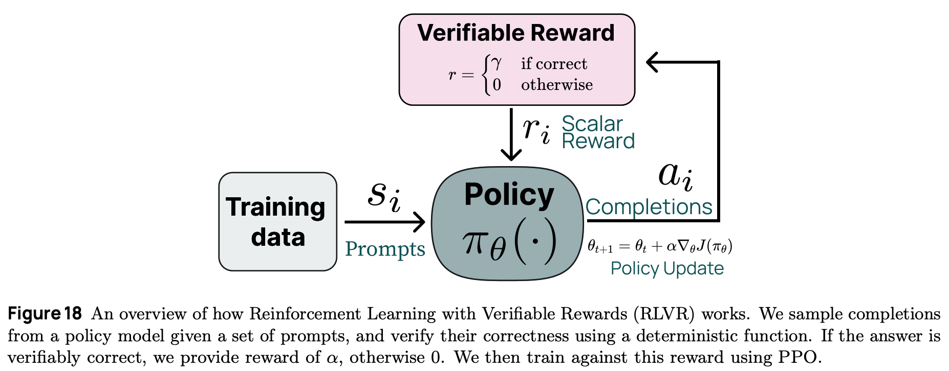
In [1], authors openly categorize Llama 4 as a “non-reasoning model”, indicating that Llama 4 is (most likely) post-training using a more standard RLHF setup—though it is still very likely that RLVR is used at least in part—and is not trained to leverage long chains of thought when solving problems. Based recent trends in LLM research, however, we should not be surprised is a reasoning-variant of Llama 4 is released in the near future. For example, DeepSeek-R1 was an extension of the previously-released DeepSeek-v3 (non-reasoning) model.

Data mixing and curation. Beyond using new algorithms, authors emphasize the importance of data curation and curriculum learning in the post-training process for Llama 4. Over 50% of the data available for SFT is removed from the training process by using an LLM judge (i.e., this is just a prior Llama model) to identify and remove easy examples, thus focusing post-training on more difficult data. For the Behemoth model, an even larger portion (95%) of this data is removed.

“We also found that dynamically filtering out prompts with zero advantage during training and constructing training batches with mixed prompts from multiple capabilities were instrumental in providing a performance boost on math, reasoning, and coding.” – from Llama 4 blog [1]

A similar strategy is used during online RL by alternating between training the model and using it to identify hard training prompts. In particular, prompt difficulty is assessed using pass@k analysis, which generates k completions with the LLM and checks how many of them are correct. Notably, a nearly identical technique is adopted by Kimi-1.5 (see Section Two of this paper) to assess prompt difficulty and develop a curriculum learning strategy. As detailed in the above quote, Llama 4 also adopts some additional tricks for identifying hard prompts and mixes data from multiple domains in each training batch to achieve a good balance in model capabilities (e.g., conversation, reasoning, coding and more).

Model Distillation

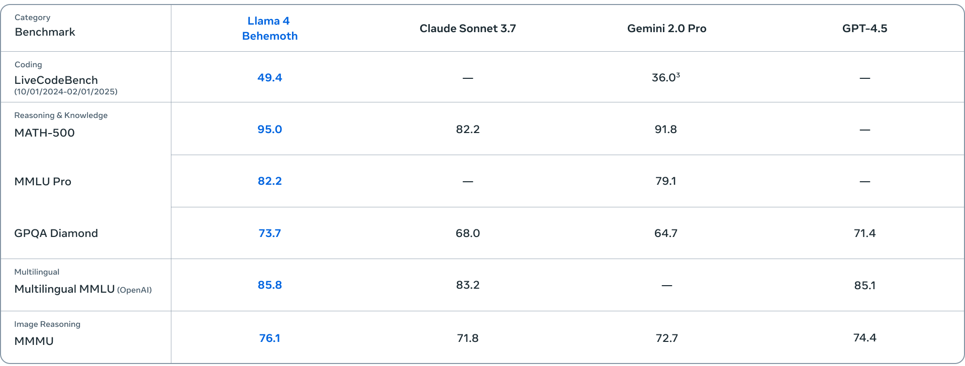
Beyond releasing the Llama 4 Scout and Maverick models in [1], authors also preview10 Llama 4 Behemoth—a much larger natively multi-modal MoE with 288B active parameters, 16 experts and 2T total parameters. The key performance metrics of the Llama 4 Behemoth model are presented in the table above.

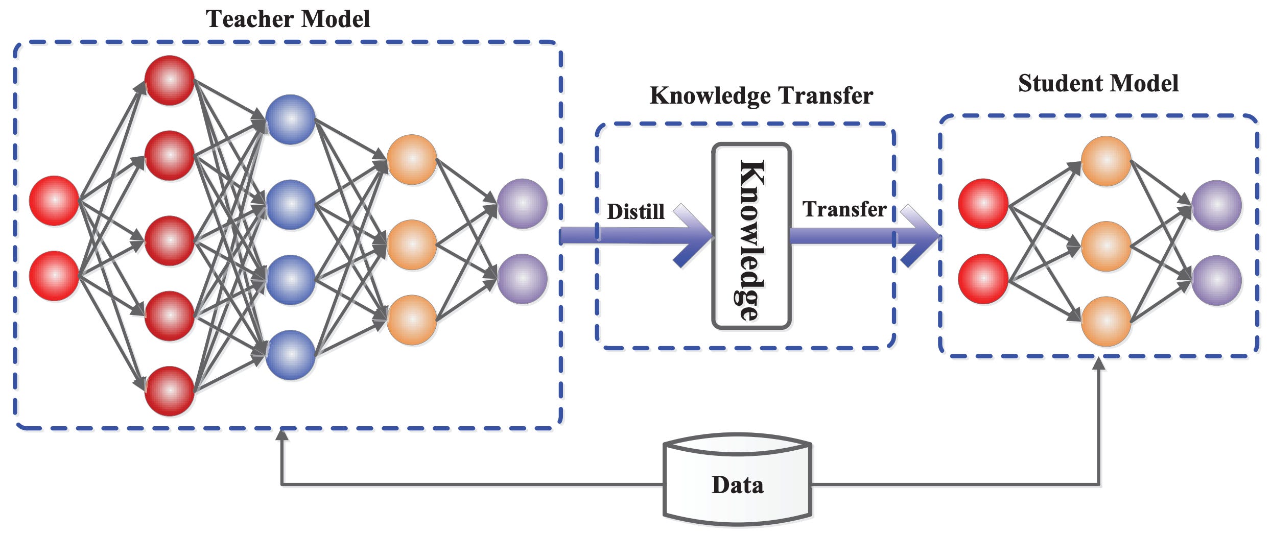
Despite the impressive performance of Llama 4 Behemoth, this model is primarily used for the purpose of knowledge distillation [15]. In other words, we use Llama 4 Behemoth as a teacher when training other Llama 4 models.

“These models are our best yet thanks to distillation from Llama 4 Behemoth, a 288 billion active parameter model with 16 experts that is our most powerful yet and among the world’s smartest LLMs.” – from Llama 4 blog [1]

What is distillation? Given a input sequence of token vectors, an LLM outputs an equally-sized set of (transformed) token vectors. We can pass each of these output vectors through the LLM’s classification-based next token prediction head—this is usually just implemented as an additional linear layer—and apply softmax to obtain a probability distribution over the set of potential next tokens. Therefore, the LLM’s final output is a list of vectors representing next token probability distributions at each position in the input sequence; see below.

import torch import torch.nn.functional as F  seq_len = 128 d = 768  # size of token embeddings vocab_size = 32678  # classification head for next token prediction ntp_head = torch.nn.Linear(in_features=d, out_features=vocab_size)  # construct LLM output and next token probabilities llm_output = torch.rand((seq_len, d)) logits = ntp_head(llm_output) ntp_probs = F.softmax(logits, dim=-1)

During training, we know what the actual next token is within the sequence. So, we can train our model using a cross-entropy loss applied to the probability of the correct next token in the sequence. This training loss is implemented below, where the ground truth next tokens at each position are stored in the target vector. Here, we provide logits as input because PyTorch already applies softmax internally within its implementation of cross-entropy.

# next token prediction (cross-entropy) loss targets = torch.randint(0, vocab_size, (seq_len,)) loss = F.cross_entropy(logits, targets)

The key idea behind knowledge distillation is deriving our target from another LLM instead of ground truth. Keeping everything else fixed, we can generate output with two LLMs—a student and a teacher—and use the teacher’s output as the target—instead of the ground truth—for training the student.

Practical examples of distillation. Knowledge distillation was proposed in the context of deep learning in [15] and has been heavily used ever since; e.g., pre-ChatGPT examples of distillation include DistilBERT and TinyViT. Distillation is also heavily used in the context of LLMs. For example, DeepSeek-v3 [16] uses the DeepSeek-R1 reasoning model [17] as a teacher during pretraining. Additionally, knowledge distillation is used to create a suite of dense reasoning models of various sizes using the massive, MoE-based DeepSeek-R1 model as a teacher. Beyond these open examples, similar strategies for distillation and synthetic data are almost certainly used for training the top closed LLMs as well. Such trends likely encouraged Meta to adopt similar approaches for Llama 4 training.

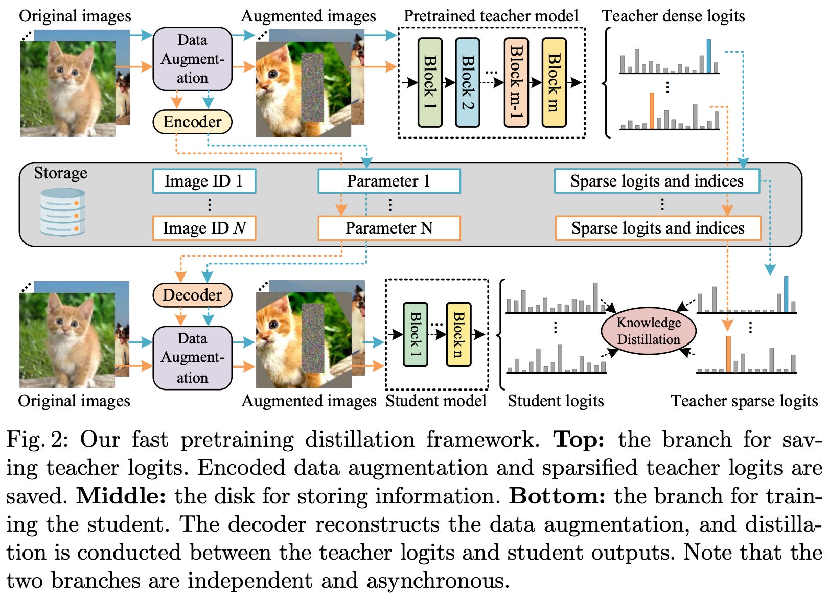
Hard vs. soft distillation. There are two main variants of knowledge distillation: hard and soft distillation. Hard distillation is very similar to our original training objective. We simply i) derive a one-hot label from the teacher LLM’s output by selecting the highest-probability token, ii) treat this one-hot label as the ground truth target and iii) apply the same cross-entropy loss; see below.

temperature = 1.0  # softmax temperature scaling_factor = 1.0  # student forward pass llm_output = torch.rand((seq_len, d)) logits = ntp_head(llm_output)  # teacher forward pass teacher_output = torch.rand((seq_len, d)) teacher_logits = ntp_head(teacher_output) teacher_ntp_probs = F.softmax(teacher_logits / temperature, dim=1)  # different distillation losses teacher_one_hot = torch.argmax(teacher_logits, dim=1) hard_loss = F.cross_entropy(logits, teacher_one_hot) soft_loss = F.cross_entropy(logits, teacher_ntp_probs) hybrid_loss = hard_loss + scaling_factor * soft_loss

However, there is a lot of potentially useful information contained within the full probability distribution predicted by the teacher model that we lose by creating the hard distillation target. Instead, we could use the entire distribution from the teacher as a training signal—this is known as soft (or dense) distillation. Such a soft distillation loss can be implemented as shown above11. Within soft distillation, we can also tweak the softmax temperature used to create the teacher’s predicted distribution of token probabilities as a training hyperparameter.

Whether to use hard or soft distillation depends on a variety of factors. For example, if we are using a closed LLM as our teacher, we may not have access to to the teacher’s logprobs, which prevents soft distillation. Assuming a powerful teacher, however, soft distillation usually provides a more dense or rich signal to the student, which speeds up training and can make the student more robust [15]. We can also use both approaches at the same time by combining them into a single loss.

Distilling Llama 4. Llama 4 models use a codistillation approach. The term “codistillation” here refers to the fact that both Llama 4 Maverick and Scout are trained using the Behemoth model as a teacher. By distilling multiple models from the larger Behemoth model, we can amortize the cost of forward passes to compute distillation targets during training, which is large—this is a big model! Authors mention in [1] that this codistillation strategy—that uses a combination of hard and soft targets—boosts the performance of both models.

“We codistilled the Llama 4 Maverick model from Llama 4 Behemoth as a teacher model, resulting in substantial quality improvements across end task evaluation metrics. We developed a novel distillation loss function that dynamically weights the soft and hard targets through training.” – from Llama 4 blog [1]

As stated above, the distillation strategy used by Llama 4 is dynamic—the balance between hard and soft targets changes throughout training. Practically, we can implement this by modifying the scaling_factor in the above code. Although the exact strategy is not revealed in [1], it is likely that the training process begins by using hard targets and emphasizes soft targets later in training, thus slowly increasing the density of information to which the LLM is exposed. This is a common form of curriculum learning, where the LLM first learns from easier data and is gradually exposed to harder data over time; e.g., see here.

Llama 4 Performance and Capabilities

LLM development is an empirically-driven and iterative process. To develop a powerful LLM, we tweak the model and build robust evaluation systems so that meaningful changes can be detected. Applying enough positive changes over time leads to a better model12. In contrast, Llama 4 makes many significant changes to the model at once—this was a complete (and risky) pivot in research direction. As we will see in this section, Llama 4 models are not state-of-the-art, and their performance was heavily criticized. However, this does not mean that the changes made by Llama 4 were a mistake. In fact, the approach taken by Llama 4 is inspired by many successful and popular LLMs. The long term success of Llama will be determined by the team’s ability to iterate and improve upon current state.

Reported Performance

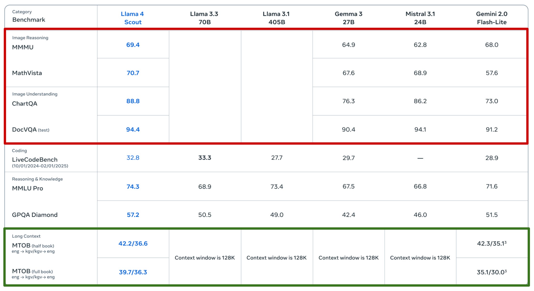
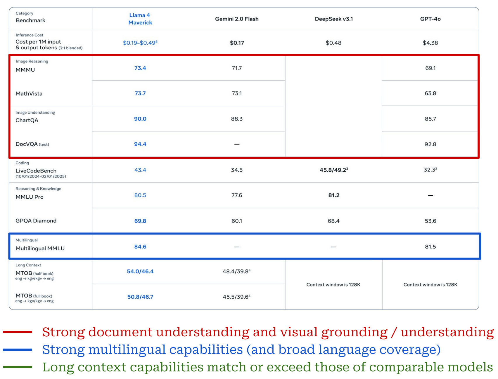
The details of benchmarks reported for Llama 4 models in [1] are summarized in the tables above, where both Llama 4 Maverick and Scout are compared to other similar models—both open and closed—on various tasks of interest. From these metrics, we see that Llama 4 models:

• Perform well on image-based document understanding tasks, likely due to the inclusion of synthetic structured images (e.g., charts, graphs and documents) in their training process.

• Have strong image understanding capabilities due to their natively multi-modal training process and early fusion architecture.

• Are more multi-lingual—meaning that more languages are supported and performance on supported languages is better—than prior Llama model iterations, as well as some closed models like GPT-4o.

• Have promising long-context capabilities, either matching or exceeding those of industry leading models like Gemini 2.0 Flash (1M token context length).

The Llama 4 Maverick model also achieves an impressive Elo score of 1417 on LMArena, which places it among the top models on the leaderboard at the time of writing. However, these results were measured with an “experimental chat version” of the model that differs from the model actually used for evaluation13.

This change caused tons of confusion and discussion online. The LMArena result was a key part of the Llama 4 release, so using a specialized model for this single evaluation was perceived as misleading (and even a bit duplicitous).

“Meta’s interpretation of our policy did not match what we expect from model providers. Meta should have made it clearer that Llama-4-Maverick-03-26-Experimental was a customized model to optimize for human preference. We are updating our leaderboard policies to reinforce our commitment to fair, reproducible evaluations so this confusion doesn’t occur in the future.” – LMArena statement

To further analyze the long context capabilities of Llama 4 models, authors in [1] also present the results of needle in a haystack tests for each model, finding that Llama 4 models are able to retrieve information from contexts up to 1M tokens (for Maverick) and 10M tokens (for Scout); see below. However, this style of long context testing only measures retrieval abilities, which do not guarantee that the model is capable of leveraging its entire context for problem solving.

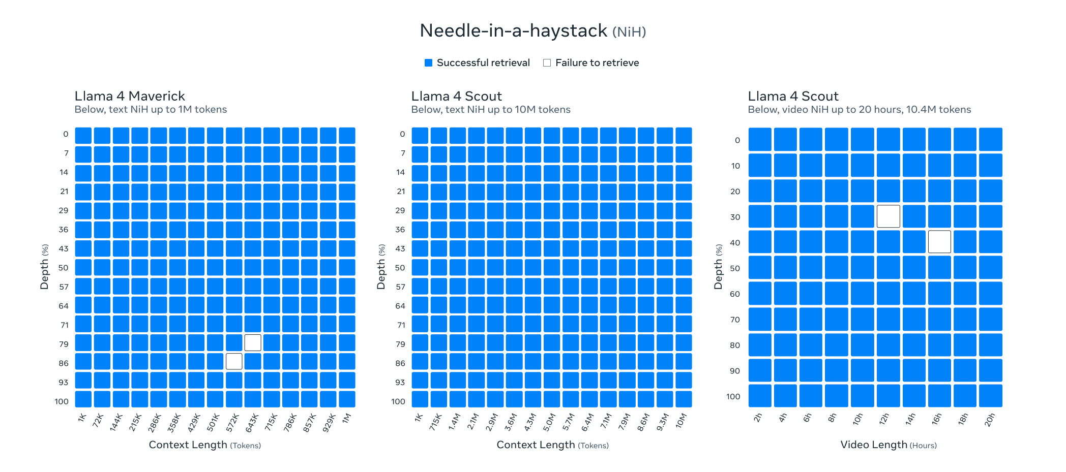
No modern long context benchmarks (e.g., BABILong, RULER or NoLiMa) are used for evaluating Llama 4, making the long context abilities of these models—one of their key distinguishing features—somewhat questionable. We also see from these metrics that Llama 4 models are not especially strong on coding tasks and—despite being strong “non-reasoning” models—are not compared to reasoning models like DeepSeek-R1 or the o-series of OpenAI models14. As we will see, the negatives do not stop here. Llama 4 models were harshly criticized after their release and public evaluations revealed many gaps in their performance.

Public Reaction and Criticism

Public evaluation. Immediately after the release of Llama 4, researchers began independently evaluating the models, and the findings were highly variable. For coding tasks, Llama 4 models definitely left something to be desired:

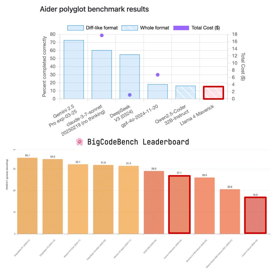
• Neither of the Llama 4 models place within the top-40 models on the BigCodeBench leaderboard [link]

• Llama 4 Maverick achieves a completion accuracy of only 16% on the Aider Polyglot benchmark (state of the art is ~80%) [link]

• Some users anecdotally published very harsh takes on the coding abilities of Llama 4 models, seeming to indicate that coding abilities were almost completely neglected in this model release [link]

These results are especially difficult to parse given that Llama 4 models do not perform poorly on all coding benchmarks; e.g., the metrics on LiveCodeBench in [1] seem to indicate reasonable coding performance.

Additionally, the long context abilities of Llama 4 models were less impressive during public evaluation; e.g., performance on the long context portion of LiveBench—a dataset with minimal data contamination—was poor. These results highlight a deeper issue with retrieval-based long context evaluations (e.g., needle in a haystack). Just because the model can retrieve information in its context does not mean it can actually leverage its entire context for problem solving.

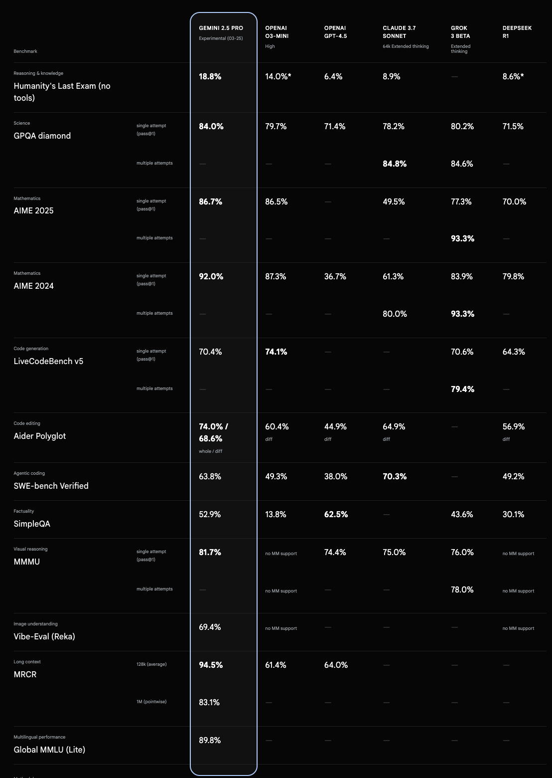
Researchers also noted that Gemini-2.5 Pro decisively outperforms even the largest Llama 4 Behemoth model on most key benchmarks; see above.

Public perception of Llama 4. The disconnect between Llama 4’s reported metrics and public evaluation results created a lot of speculation and frustration within the AI research community, even leading to false claims that testing data was purposefully included in Llama 4’s training dataset to inflate benchmark scores. These claims were quickly denied by Meta executives, who emphasized that fluctuations in model performance are due to implementation differences within the model itself, quantization strategies for inference, and more.

Nonetheless, the confused aura around the release of Llama 4 remains. Many aspects of this release were seemingly rushed, beginning with the random decision to release the model on a Saturday instead of the following Monday.

The Future of Llama

The release of Llama 4 was received poorly by the AI research community. Now that we have a deep understanding of these models, however, we see that the story behind Llama 4 is nuanced. Relative to Llama 3, these new Llama models modify—or completely reinvent—nearly every component of the model:

• MoE-based model architecture.

• Different approach to multi-modality (early fusion).

• Natively multi-modal pretraining.

• Emphasis on model distillation during pretraining.

• Completely different post-training pipeline.

• Focus on long context capabilities.

The open LLM landscape is becoming more competitive with the success of DeepSeek-v3, Qwen-2.5 and more. With the release of Llama 4, Meta both responded to this competition and made clear their goal of creating a frontier-level Llama model. Llama 4 does not achieve this goal, but this should not come as a surprise. Meta took an (obvious) risk—which may still prove to be the correct choice in the long run—by pivoting in their research strategy.

Frontier-Level Llama Models. Given the staggering pace of LLM research, the success of Llama is far from guaranteed, and Meta has a lot of work to do after falling short with Llama 4. To create a frontier-level LLM, Meta needs to iterate and improve upon their models more quickly. Those who work closely with Llama models might have noticed that the amount of time between major Llama releases has been slowly increasing:

• Llama was released in February 2023.

• Llama 2 was released in July 2023.

• Llama 3 was released in April 2024.

• Llama 4 was released in April 2025.

This expanding gap is worrying and lags behind top labs; e.g., since January 2024 DeepSeek has released DeepSeek-v1, v2, v3 and R1. Even if the next Llama model is state-of-the-art, new models will be released shortly after. Models will continue to evolve and improve at an uncomfortable pace. The only way forward is to iterate quickly and fix the gaps in evaluation capabilities that led to the huge disconnect between internal and external evaluations of Llama 4.

The Open LLM Landscape. Even if Llama models are not state-of-the-art, they can still be successful in the open LLM landscape, where many other factors—like barrier to entry and ease of use—are important. To maximize success, Meta must do everything they can to avoid restricting use cases for open LLMs. Most notably, Llama 4 models need to be distilled into a variety of smaller, dense models—in a similar fashion to DeepSeek-R1 and Qwen-2.5—to avoid the hardware requirements of massive MoEs. Creating a frontier-level Llama model is an important goal, but it should not come at the cost of deteriorating Meta’s position in the open LLM landscape. After all, Llama has never been the top-performing LLM. The emphasis upon openness is what made Llama successful in the first place.

New to the newsletter?

Hi! I’m Cameron R. Wolfe, Deep Learning Ph.D. and Senior Research Scientist at Netflix. This is the Deep (Learning) Focus newsletter, where I help readers better understand important topics in AI research. If you like the newsletter, please subscribe, share it, or follow me on X and LinkedIn!

Subscribe now

Bibliography

[1] Meta. “The Llama 4 herd: The beginning of a new era of natively multimodal AI innovation” https://ai.meta.com/blog/llama-4-multimodal-intelligence/ (2025).

[2] Grattafiori, Aaron, et al. “The llama 3 herd of models.” arXiv preprint arXiv:2407.21783 (2024).

[3] Liu, Aixin, et al. “Deepseek-v2: A strong, economical, and efficient mixture-of-experts language model.” arXiv preprint arXiv:2405.04434 (2024).

[4] Liu, Aixin, et al. “Deepseek-v3 technical report.” arXiv preprint arXiv:2412.19437 (2024).

[5] Guo, Daya, et al. “Deepseek-r1: Incentivizing reasoning capability in llms via reinforcement learning.” arXiv preprint arXiv:2501.12948 (2025).

[6] Team, Chameleon. “Chameleon: Mixed-modal early-fusion foundation models.” arXiv preprint arXiv:2405.09818 (2024).

[7] Bavishi, Rohan, et al. “Fuyu-8b: A multimodal architecture for ai agents.” URL: https://www. adept. ai/blog/fuyu-8b (2023).

[8] Xiong, Ruibin, et al. “On layer normalization in the transformer architecture.” International conference on machine learning. PMLR, 2020.

[9] Xu, Hu, et al. “Demystifying clip data.” arXiv preprint arXiv:2309.16671 (2023).

[10] Blakeney, Cody, et al. “Does your data spark joy? Performance gains from domain upsampling at the end of training.” arXiv preprint arXiv:2406.03476 (2024).

[11] Su, Jianlin, et al. “Roformer: Enhanced transformer with rotary position embedding.” Neurocomputing 568 (2024): 127063.

[12] Kazemnejad, Amirhossein, et al. “The impact of positional encoding on length generalization in transformers.” Advances in Neural Information Processing Systems 36 (2023): 24892-24928.

[13] Nakanishi, Ken M. “Scalable-Softmax Is Superior for Attention.” arXiv preprint arXiv:2501.19399 (2025).

[14] Lu, Yi, et al. “A controlled study on long context extension and generalization in llms.” arXiv preprint arXiv:2409.12181 (2024).

[15] Hinton, Geoffrey, Oriol Vinyals, and Jeff Dean. “Distilling the knowledge in a neural network.” arXiv preprint arXiv:1503.02531 (2015).

[16] Liu, Aixin, et al. “Deepseek-v3 technical report.” arXiv preprint arXiv:2412.19437 (2024).

[17] Guo, Daya, et al. “Deepseek-r1: Incentivizing reasoning capability in llms via reinforcement learning.” arXiv preprint arXiv:2501.12948 (2025).

[18] Rafailov, Rafael, et al. “Direct preference optimization: Your language model is secretly a reward model.” Advances in Neural Information Processing Systems 36 (2023): 53728-53741.

[19] Tang, Yunhao, et al. “Understanding the performance gap between online and offline alignment algorithms.” arXiv preprint arXiv:2405.08448 (2024).

Deep (Learning) Focus