In this article, we’ll explore “Disentangled Variational Autoencoders”, an AI strategy for breaking complex data down into its fundamental parts.

“Autoencoders” are an essential AI building block that allows data scientists to compress data into its essential components automatically. Autoencoders are vital in tasks like image segmentation, error correction, and audio processing.

“Variational” autoencoders, and “Disentangled” autoencoders are modifications to the traditional autoencoder design that encourage autoencoders to produce output that is both more useful and better human interpretable.

In this article, we’ll start by forming a thorough understanding of the traditional autoencoder, develop that understanding further by exploring variational autoencoders, and then conclude by discussing disentangled variational autoencoders.

Who is this useful for? Anyone interested in forming a complete understanding of AI

How advanced is this post? This article is conceptually accessible to all readers, especially the earlier sections. The implementation sections are geared to data scientists with PyTorch experience.

Prerequisites: None, from a conceptual level, but it would likely be beneficial to have some theoretical AI understanding before reading this article. I have a few articles listed below which may serve as good supplementary reading.

The description of variational autoencoders also assumes some basic statistics knowledge, chiefly around understanding normal distributions, mean, standard deviation, and gaussians. I’m working on a piece describing fundamental statistical ideas, so stay tuned.

Dimensionality

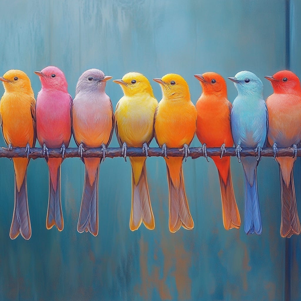
Conceptually, everything we’ll be discussing hinges on the concept of “dimensionality”, meaning “how many ways it takes to describe a thing”. For instance, take the following image:

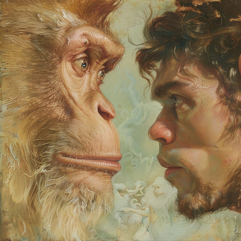
This image can be described in several ways:

• The image can be described completely by listing each pixel in the image.

• The image can be described as a downsampled version of the image, where we get all the fundamental structure but lose some detail.

• The image can be described with the text “an ape on the left, and a guy on the right, looking at each other”.

• The image can be described with the text “an AI-generated painting”.

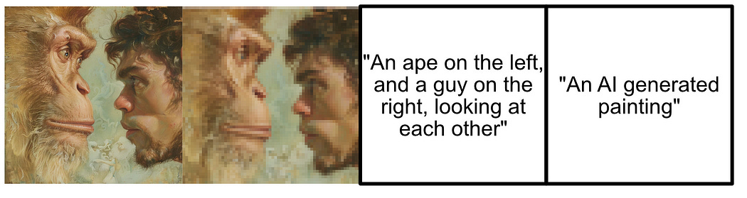
Each of these representations of the image is valid but with a different degree of resolution. Intuitively, from left to right, one might consider each successive representation to be less completely defined.

This is somewhat similar to the idea of image compression. A high-resolution image is very large in terms of its memory footprint, so the idea of image compression is to represent an image in a form that takes up less data, but that can be decoded into a similar, if not identical image.

As data scientists, this idea of “representing the same fundamental thing but with less data” is incredibly compelling. Data like images and audio have a ton of information, which means we need very large and complex models to deal with the data effectively. If we could distill this data into a smaller yet fundamentally equivalent representation, we might be able to leverage that to build performant and efficient AI systems.

The idea of an autoencoder is to build a model that can compress data into a more fundamental representation, kind of like how image compression works, so we can use those distilled representations for all sorts of clever tasks.

The AutoEncoder, and Dimensionality Reduction

The idea of the autoencoder started way back in the early days of artificial intelligence, with Learning Internal Representations by Error Propagation.

This paper was most famous for its impact in popularizing backpropagation, a fundamental AI algorithm. For us, though, it’s immediately relevant because, even in this bedrock paper, the idea of using AI models to compress and decompress information was at the forefront.

The fundamental idea of using AI to compress data has existed, essentially, for as long as modern AI has existed. Throughout the early decades of modern AI, the idea of the autoencoder emerged not as a single event, but as a general elaboration on using AI to compress and decompress data.

This amorphous beginning makes autoencoders a bit challenging to write about because the autoencoder didn’t really have an explicit beginning. It’s more of a general idea that has been retroactively coined.

Essentially, though, an autoencoder is a model that’s designed to be able to compress and decompress an input through the usage of a “bottleneck”. To better understand what that really means, I think it might be useful to work through a simple example.

A Simple AutoEncoder

We’ll be covering a few styles of autoencoders throughout this article. Let’s start with the prototypical autoencoder, which is very much in line with the models defined in Learning Internal Representations by Error Propagation.

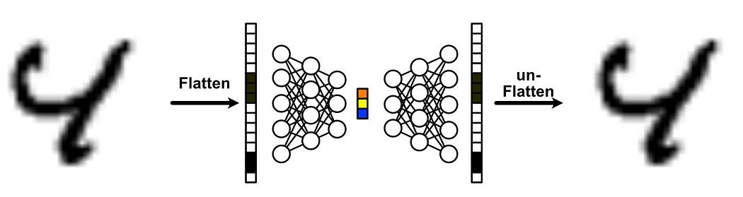
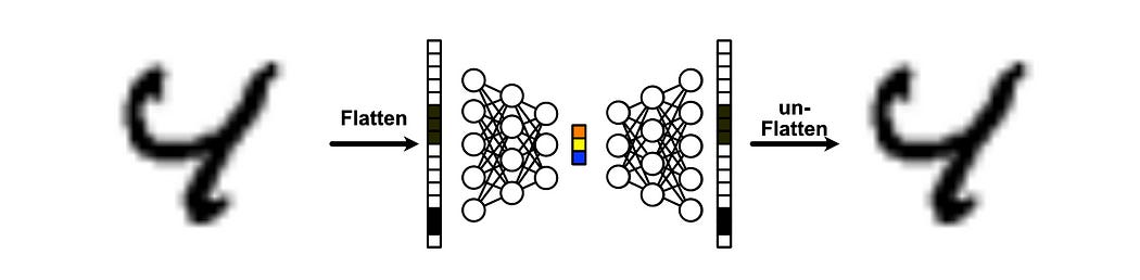
This takes the form of a neural network, which accepts some input, and crunches that data into something called an “information bottleneck” before then building the data back up into an output.

We can use MNIST as an example of how this might work. MNIST is a fundamental toy problem in artificial intelligence, which consists of many images of hand drawn digits.

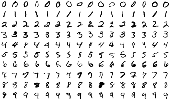
If we flatten out each image into a vector, we can use a neural network to compress that data down into a small representation, and then use another neural network to decompress that data into a similar image we started with.

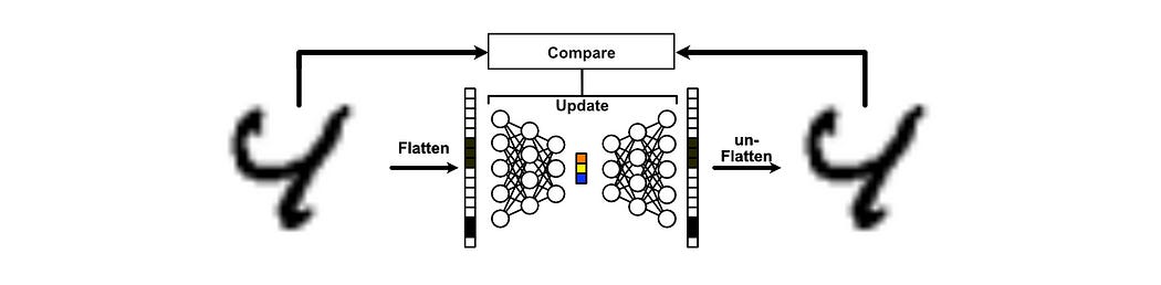
We’ll train this model by giving it a bunch of input images, then update the model based on how well it reconstructed the original image. After numerous rounds of training the model based on various inputs, the autoencoder should get better at the task of compressing and decompressing images.

By modern definitions, this is a prototypical autoencoder. It consists of three fundamental components:

• Encoder: Compresses the input into a smaller representation.

• Latent Embedding: The compressed representation produced by the encoder.

• Decoder: Reconstructs the original input from the latent embedding.

Let’s whip it up in code. Full code can be found here.

First, we need to load up the MNIST dataset and import a few dependencies.

import torch import torch.nn as nn import torchvision import torchvision.transforms as transforms from torch.utils.data import DataLoader  transform = transforms.ToTensor() train_dataset = torchvision.datasets.MNIST(root='./data', train=True, transform=transform, download=True) train_loader = DataLoader(train_dataset, batch_size=128, shuffle=True)

Then, we can go straight into defining our autoencoder.

class Autoencoder(nn.Module):     def __init__(self):         super().__init__()         self.encoder = nn.Sequential(             nn.Linear(28*28, 128),             nn.ReLU(True),             nn.Linear(128, 64),             nn.ReLU(True),             nn.Linear(64, 32)         )         self.decoder = nn.Sequential(             nn.Linear(32, 64),             nn.ReLU(True),             nn.Linear(64, 128),             nn.ReLU(True),             nn.Linear(128, 28*28),             nn.Sigmoid()         )      def forward(self, x):         x = x.view(x.size(0), -1)  # Flatten         encoded = self.encoder(x)         decoded = self.decoder(encoded)         return decoded.view(x.size(0), 1, 28, 28)

In the MNIST dataset, each image consists of a 28×28 pixel grid. When we pass that image to our model, we first project that 2D grid into a 1D vector using x.view(x.size(0), -1). This results in a vector of length 748.

The encoder then passes the input through sequentially smaller layers, trimming the initial 748 dimensions input into 128, then 64, then finally 32. The encoded representation, thus, is only 4% of the size of the original input.

We then pass that encoded representation to the decoder, which builds up the representation from 32, to 64, to 128, to 748. This is then reformatted back into a 28×28 grid via decoded.view(x.size(0), 1, 28, 28).

The ReLU activation functions are used to sprinkle some non-linearity in the mix, and Sigmoid is used to ensure the final output for each pixel is between 0 (black) and 1 (white).

We can then train this model, pretty much like any other neural network.

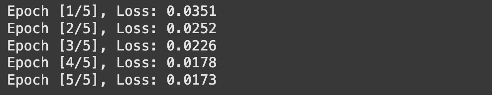
device = torch.device('cuda' if torch.cuda.is_available() else 'cpu') model = Autoencoder().to(device) criterion = nn.MSELoss() optimizer = torch.optim.Adam(model.parameters(), lr=1e-3) num_epochs = 5 for epoch in range(num_epochs):     for img, _ in train_loader:         img = img.to(device)         output = model(img)         loss = criterion(output, img)         optimizer.zero_grad()         loss.backward()         optimizer.step()     print(f'Epoch [{epoch+1}/{num_epochs}], Loss: {loss.item():.4f}')

going line by line:

1. first, we’re figuring out if there’s a GPU available or not

2. Then we’re making a new instance of our Autoencoder model and putting it on that device

3. We’re then defining our “criterion”, probably the most complex idea in this code block. MSELoss stands for “mean squared error loss”. This is a function that gives us a big number if our two inputs are different, and a small number if our two inputs are the same. We’ll be using this to compare if our input and output images are similar.

4. we’re defining an optimizer. This is the thing that updates parameters based on errors in PyTorch.

5. with num_epochs set to 5, that means we’re going through all of our training data in MNIST 5 times.

6. this is our actual epoch loop

7. this is our iteration through all the data in the training data

8. we put the image data on whatever device we’re using, GPU or CPU (critically, the same device the model is on).

9. we pass the image through our model, thus passing it through both the encoder and decoder. This results in the autoencoder’s reconstruction of the image

10. we compare the original image to the output image, with our mean squared error loss function, to get a number. If this is a big number, that means the model did a bad job.

11. optimizer.zero_grad() resets our optimizer to get it ready for a new iteration.

12. loss.backward() triggers back-propagation, which essentially goes through the model and calculates how it should update to be less bad than the example we just passed through.

13. optimizer.step() updates the parameters of the model based on the results of loss.backward()

14. printing out stuff, for bookkeeping.

If a lot of that was very new to you, I highly recommend my article on AI for the novice, which covers AI in PyTorch from first principles, assuming no prior knowledge.

If we run that code, we’ll see the loss is steadily declining, meaning the autoencoder output is becoming more and more similar to the input over successive iterations.

We can then visualize a few examples of inputs, encoded representations of those inputs, and re-constructed outputs to get an idea of what our autoencoder is doing.

import matplotlib.pyplot as plt  # Set model to eval mode model.eval()  # Choose n random examples n = 6 examples = next(iter(DataLoader(train_dataset, batch_size=n, shuffle=True))) images, _ = examples images = images.to(device)  # Forward pass with torch.no_grad():     flat_images = images.view(images.size(0), -1)     latents = model.encoder(flat_images)     reconstructions = model.decoder(latents).view(-1, 1, 28, 28)  # Plot in a 3-column grid: Original | Latent | Reconstructed fig, axes = plt.subplots(nrows=n, ncols=3, figsize=(9, 2.5 * n))  for i in range(n):     # Column 1: Original     axes[i, 0].imshow(images[i].cpu().squeeze(), cmap='gray')     axes[i, 0].set_title("Original", fontsize=10)     axes[i, 0].axis('off')      # Column 2: Latent representation as 1D heatmap     axes[i, 1].imshow(latents[i].cpu().view(1, -1), cmap='viridis', aspect='auto')     axes[i, 1].set_title("Latent Vector", fontsize=10)     axes[i, 1].axis('off')      # Column 3: Reconstructed     axes[i, 2].imshow(reconstructions[i].cpu().squeeze(), cmap='gray')     axes[i, 2].set_title("Reconstruction", fontsize=10)     axes[i, 2].axis('off')  # Shared y-label for readability for ax in axes[:, 0]:     ax.set_ylabel("Sample", fontsize=10)  plt.tight_layout() plt.show()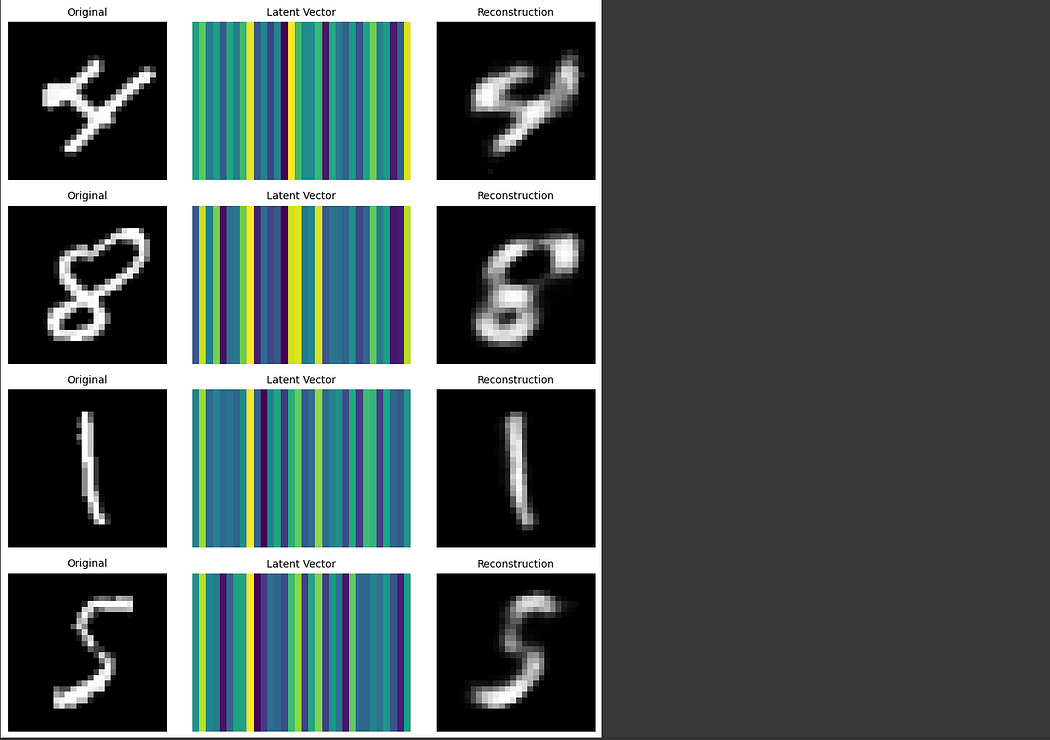

Here, we’re passing images into the encoder, visualizing the latent encoded representation from the encoder (which is comprised of 32 values), then visualizing the reconstruction from the decoder.

And that’s the autoencoder, in its simplest sense. We’ll talk about “variational” and “disentangled” autoencoders in future sections, but I quickly want to discuss some of the applications of the autoencoder to get an idea of why the overall concept is applicable in the first place.

A Few Applications

Autoencoders are used all over the place. In fact, the reason I’m covering them now is because I plan on covering a few advanced AI approaches that leverage autoencoders within their greater architecture. Things like voice synthesis, diffusion, and using AI to decode images based on brain waves. Pretty crazy stuff. For now, though, I think we can start with a simple application: denoising.

Denoising

Recall that, in the previous section, we trained an encoder and decoder to construct a perfect recreation of the original image. Of course, it wasn’t perfect, but that was the objective: the model was updated on the MSELoss between the input and output images.

With a minor adjustment, we can turn this into a de-noising model. Instead of putting the original image in the input, we can put in a version of the image with some random noise added to it. Then, we can train our model based on the difference of the output with the input without noise. Thus, the model is trained to create a reconstruction that doesn’t have noise.

This is achievable with a very simple modification to our training code. Instead of putting our image in as the input, we apply some noise to the image before feeding it into the model.

# 1. Add noise function def add_noise(inputs, noise_factor=0.5):     noisy = inputs + noise_factor * torch.randn_like(inputs)     return torch.clip(noisy, 0., 1.)  # Keep pixel values in [0,1]  # 2. Denoising training loop num_epochs = 5 noise_factor = 0.5  for epoch in range(num_epochs):     model.train()     total_loss = 0      for img, _ in train_loader:         img = img.to(device)         noisy_img = add_noise(img, noise_factor=noise_factor)          # Forward pass         output = model(noisy_img)         loss = criterion(output, img)  # Compare to clean target          # Backprop and optimize         optimizer.zero_grad()         loss.backward()         optimizer.step()                  total_loss += loss.item()      avg_loss = total_loss / len(train_loader)     print(f"[Epoch {epoch+1}/{num_epochs}] Loss: {avg_loss:.4f}")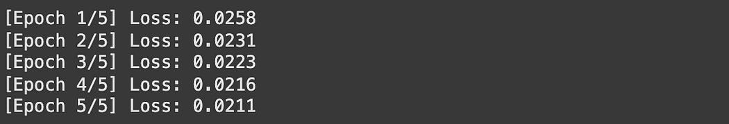

As you can see, the loss is a bit higher, which makes sense because this is a more difficult problem. Still, there is some convergence going on. Let’s visualize some output to see what we get.

import matplotlib.pyplot as plt  # Set to evaluation mode model.eval()  # Get n random samples n = 6 examples = next(iter(DataLoader(train_dataset, batch_size=n, shuffle=True))) images, _ = examples images = images.to(device)  # Add noise noisy_images = add_noise(images, noise_factor=0.5)  # Denoise with torch.no_grad():     denoised_images = model(noisy_images)  # Plot: Noisy → Denoised → Original fig, axes = plt.subplots(nrows=n, ncols=3, figsize=(9, 2.5 * n))  for i in range(n):     # Noisy Input     axes[i, 0].imshow(noisy_images[i].cpu().squeeze(), cmap='gray')     axes[i, 0].set_title("Noisy Input", fontsize=10)     axes[i, 0].axis('off')      # Denoised Output     axes[i, 1].imshow(denoised_images[i].cpu().squeeze(), cmap='gray')     axes[i, 1].set_title("Denoised Output", fontsize=10)     axes[i, 1].axis('off')      # Original Image     axes[i, 2].imshow(images[i].cpu().squeeze(), cmap='gray')     axes[i, 2].set_title("Original Image", fontsize=10)     axes[i, 2].axis('off')  plt.tight_layout() plt.show()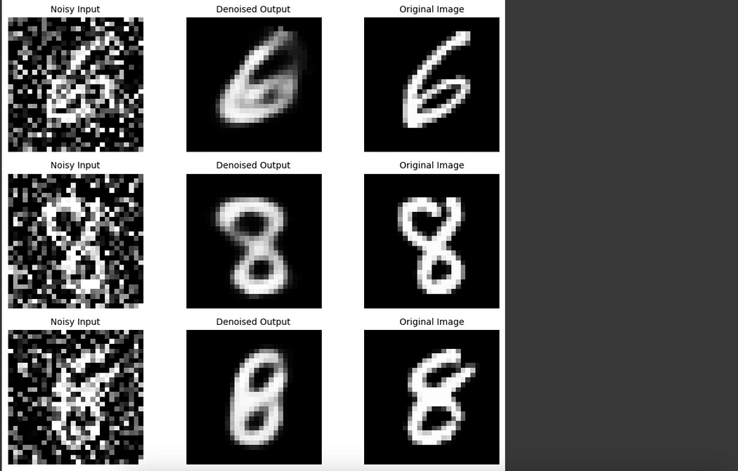

And, ta-dah, with a minor modification we’ve made a simple de-noising model.

This is a bit of an interesting adjustment to the original autoencoder we discussed. The model has the same architecture, but because we modified the training objective we can think of the encoder and decoder slightly differently. You can think of the encoder job as denoising, trying to summarize the noisy input into a vector representation that summarizes the core ideas of the image, and you can think of the decoder as a projection that then constructs an image based on that summarization.

This general idea is very popular, especially in computer vision. Check out my article on Projection Heads, which elaborates on this general idea further.

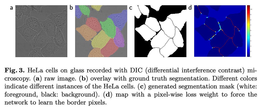
Image Segmentation with U-Nets

While the original ideas of the autoencoder were centered around a traditional multilayered neural network, modern autoencoders often employ different underlying architectures. Convolutional U-Net models, for instance, can be thought of as a flavor of autoencoder.

For the more novice readers, convolution is a type of neural network that employs a series of filters and down-samplers. This is particularly useful in images because you don’t need to learn a parameter for each pixel, rather you learn parameters in a filter that gets applied to pixels.

A U-Net architecture uses convolutions and down-sampling techniques to convert an image into a low-dimensional representation, the objective being to force the model to create a distilled representation of the entire image. Then, there is another side to the U-Net which upsamples from that compressed representation. There’s some other stuff going on in U-Nets, but you can think of them as a flavor of autoencoder.

These are a great, practical model for performing complex operations on images, like image segmentation.

We’ll be sticking with neural networks in this article, but it’s important to note that a variational autoencoder doesn’t necessarily have to be a classic neural network. It can be a convolutional network, LSTM, transformer, or whatever.

Variational Autoencoders (VAEs)

Autoencoders are great in a lot of applications, but they have one serious drawback: their encoded representations have a tendency to make little to no sense.

Recall, in a previous example, we used a simple autoencoder to reconstruct images of numbers

A natural question might be, what do the values in the latent vector actually represent? Do these values make some level of sense to a human? Is there a spot in the vector that might, for instance, allow us to blend between a 1 and a 7? Does another spot in the vector represent how tilted the number is? perhaps another spot in the vector encodes how curved the bottom of a character is, distinguishing between a 5 and an 8?

Unfortunately, vanilla autoencoders are very bad at creating representations that obey any reasonable rules. If you start playing around with the latent representation of some input, you almost certainly will get gibberish as output, rather than some ability to blend between features that a human would care about.

The goal of a variational autoencoder (VAE) is to attempt to make the latent vectors obey some reasonable rules. Instead of a bunch of vague values, A variational autoencoder is designed to promote the creation of distributions in the latent encoding, such that one can “blend between” different types of inputs.

With normal autoencoders, it’s hard to use the latent representation for anything useful, but because variational autoencoders are designed to have latent encoded representations that have smooth, reasonable transitions between important features in the underlying data, it allows these representations to be used more effectively, both by humans and other AI models (We’ll be elaborating on that in a bit).

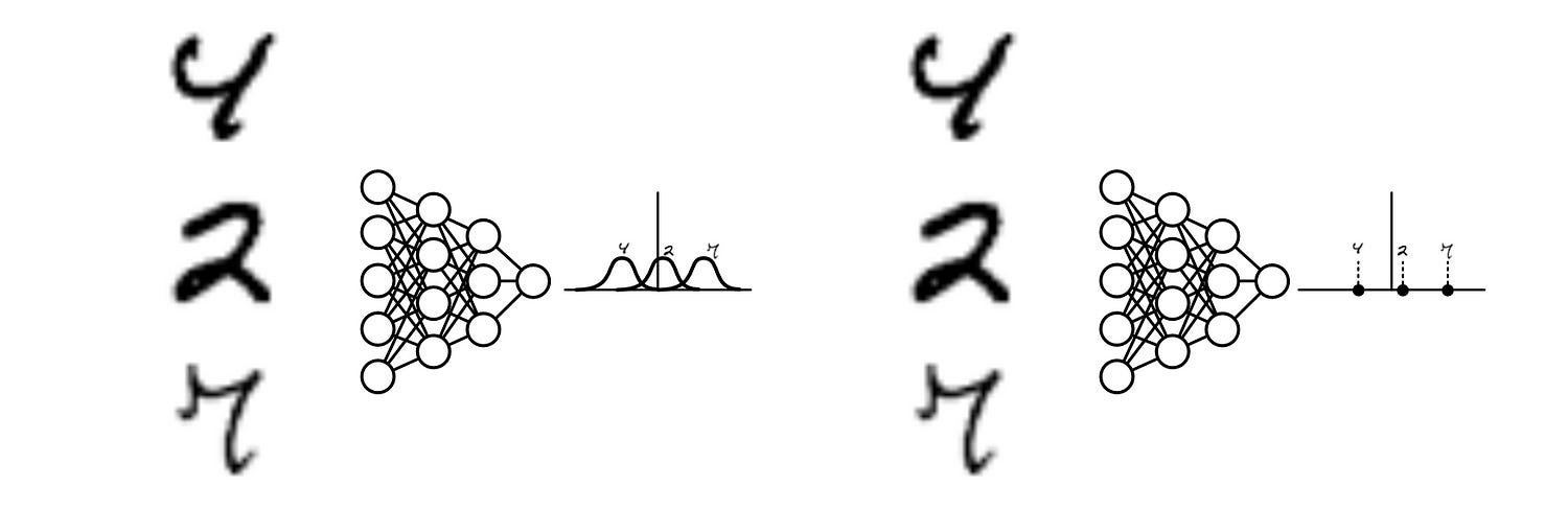
Variational autoencoders are very similar to the traditional autoencoder, save one key difference. Variational autoencoders use distributions in their intermediate representation, rather than vectors.

Recall, in the traditional autoencoder, the encoder outputs a vector which the decoder uses to construct the output.

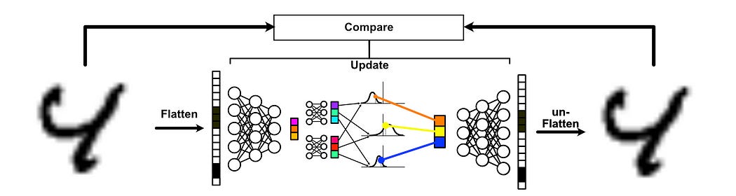
In a variational autoencoder, the encoder instead outputs a set of probability distributions. Those distributions are then sampled, and that sample is fed to the decoder to construct the output.

In other words, with variational autoencoders, an input isn’t mapped to a point, it’s mapped to a region, which is defined by a probability distribution. The encoder learns to move around these probability distributions throughout the training process, and thus learns to organize the data into regions that make some level of sense.

Because the encoder outputs a “region” from a given input, rather than a deterministic vector of values, the encoder and decoder must work together throughout the learning process to have a “smoother” understanding of the problem. Instead of hyper-specific combinations of values that need to be aligned just right to create a good output from the decoder, VAEs tend to make more robust latent representations that smoothly blend between important characteristics in the data.

The Math of Variational Autoencoders

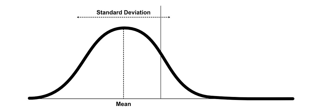
At its most fundamental, Variational autoencoders are much like the traditional autoencoder, but variational autoencoders replace the latent vector with two vectors, one for mean, and the other for standard deviation.

This allows us to define something called a “gaussian”, or “normal distribution” for each value in the latent vector.

When we pass data through a variational autoencoder, we construct these gaussians based on the input, sample from that distribution, pass the sample to the decoder, and construct our output. We then update the model to produce better gaussians that are less wrong.

To make this a bit more intuitive, it’s helpful to imagine a very small dataset being passed to the variational autoencoder. Let’s say we had a dataset of three images, and the variational autoencoder had a latent dimension of just one value. So the encoder compresses the data down to a single number, which the decoder needs to expand to produce the output.

If we pass this data, over and over again over many epochs, through our variational autoencoder, the same data will end up creating different latent vectors because each time the vector is sampled from the region generated from that input. Thus, the variational autoencoder is forced to organize these regions so that they’re separate from one another. This is much more sophisticated than the traditional autoencoder, which might simply settle on the number -0.5 representing the first image, the number 0.1 representing the second image, and 0.8 representing the third image.

The astute among you might think “Why wouldn’t the variational autoencoder do that anyway”. The whole idea of the variational autoencoder is that it learns by manipulating these distributions to separate inputs for reconstruction. Wouldn’t it be best for it to simply collapse all the distributions to a very small size and separate them as much as possible, thus practically becoming equivalent to the traditional autoencoder?

In many applications, yes. To fight this tendency, and promote smooth distributions in the variational autoencoder, a concept called “KL Divergence” is applied to the loss function during training.

KL Divergence is a way to mathematically define how different two distributions are. If two distributions perfectly overlap, ther KL divergence is zero. As they begin to deviate from one another, their KL divergence increases.

It’s used a lot when you want to constrain an AI model to obey some rule. For instance, DeepSeek-R1 uses it a lot in its training strategy, “Group Relative Policy Optimization”, which is a mountain I have yet to fully summit (I blew a few hundred bucks on GPUs without getting it to work… It’s still a work in progress, if you’re not a paying member please consider supporting IAEE!) I do cover the concept in my article on DeepSeek, though.

For Variational Autoencoders, KL Divergence is used to penalize the model any time any of its gaussiens deviate from a standard gaussian of a mean of 0 and a standard deviation of 1. The more they deviate, the larger the penalty. As the model learns to organize distributions to separate inputs from one another, it gets penalized for having a larger KL Divergence. Thus the model is forced to learn to balance robust output with a bias for overlapping distributions.

The VAE paper has a ton of complicated math, but it all ends up boiling down to a single function.

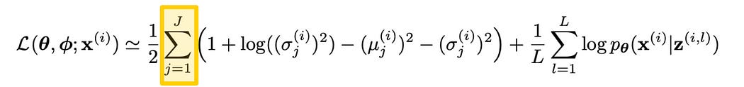
This is the loss function of the variational autoencoder, which dictates how the model is trained and thus functions. In actuality this isn’t a loss function in the conventional sense, because in this paper the objective is to maximize, rather than minimize this expression. If you wanted it to be a true loss function, you would just multiply the whole thing by -1.

The loss function “L” accepts three inputs

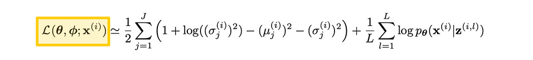
• θ (theta) is the parameters of the decoder

• ϕ (phi) is the parameters of the encoder

• x(i) is a particular input (i.e. image) out of the dataset.

One subtlety that might throw you through a loop is the existence of a semicolon (;) in the arguments. Normally, a comma (,) is used to distinguish between arguments of a function, but the semicolon can be used to distinguish between different types of inputs. θ and ϕ are model parameters, while x(i) is training data. Thus a semicolon was used to note that these are different types of data.

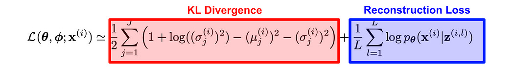
Then we get to the meat of the equation. The loss function for variational autoencoders consists of two sub-expressions. One is the KL Divergence (which restricts how far the output gaussians can deviate from a standard gaussian), and another expression that evaluates the reconstruction quality of the final output.

The KL divergence has all sorts of fancy subtle math details, some of which we’ll dive into and some of which we’ll leave to theory. From its highest level, it penalizes distributions that are not like the standard gaussian.

First of all, any mean which is not zero results in a penalty. This makes sense because the whole point of KL divergence is to penalize deviation from a normal distribution with a mean of zero. Recall that we’re trying to maximize this particular loss function, so subtracting by the square of the mean (which is always positive) would result in a penalty for all values besides a mean of zero.

How KL Divergence handles standard deviation (σ, sigma) is a bit more complicated. The name of the game is to penalize distributions that are smaller or bigger than a standard deviation of 1.

If we print out 1+log(σ²)-σ², we get the following graph:

The justification for why it’s written this way is… A bit complex for my liking. It has to do with ideas of information entropy, log variance, and all sorts of other complicated stuff. Frankly, I’m not interested in spending hours of my time on all the nitty gritty details. Because of the way this expression is formulated, a sigma value of 1 results in the best value relative to the loss function, with all other possible sigma values resulting in less desirable output. I expect there are many similar ways one could express this function which would result in a similar effect, but this is the one the researchers settled on because of complicated theoretical reasons. It also looks nice and is fairly elegant, which is cool.

So, that’s the KL divergence portion of the loss function. All the distributions within the model are penalized for deviating from a mean of zero and a standard deviation of 1. Now we can shift to discussing the reconstruction loss portion of the equation.

To fully understand this equation, it’s helpful to bring in a few definitions from the VAE paper, which describe a famous detail of the VAE paper called the “reparameterization trick”

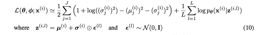
Recall, from a high level, the VAE outputs a vector of distributions (in the form of means and standard deviations) and then samples from that distribution to generate an output. This is what makes the VAE better at smooth and interpretable latent representations. Well, there’s a serious problem with sampling from a distribution: it’s not differentiable.

Modern ML models rely on an ability to trace back from the output to the input, and update all the parameters in the model to make the output better. In order for AI to work, you need to be able to say “This pixel should have been lighter, so all the parameters need to update in this way to make that pixel brighter”. This is how AI models learn, and is called “back propagation”, which I discuss in depth in the following articles:

Randomly sampling from a distribution breaks this strong connection traced between the output and the input, meaning we can’t train our encoder because it happens before sampling occurs.

The reparameterization trick gets around this problem by separating sampling from the model. Instead of sampling from a distribution defined by the model, we sample from a separate distribution and then scale that sample by the parameters in the model.

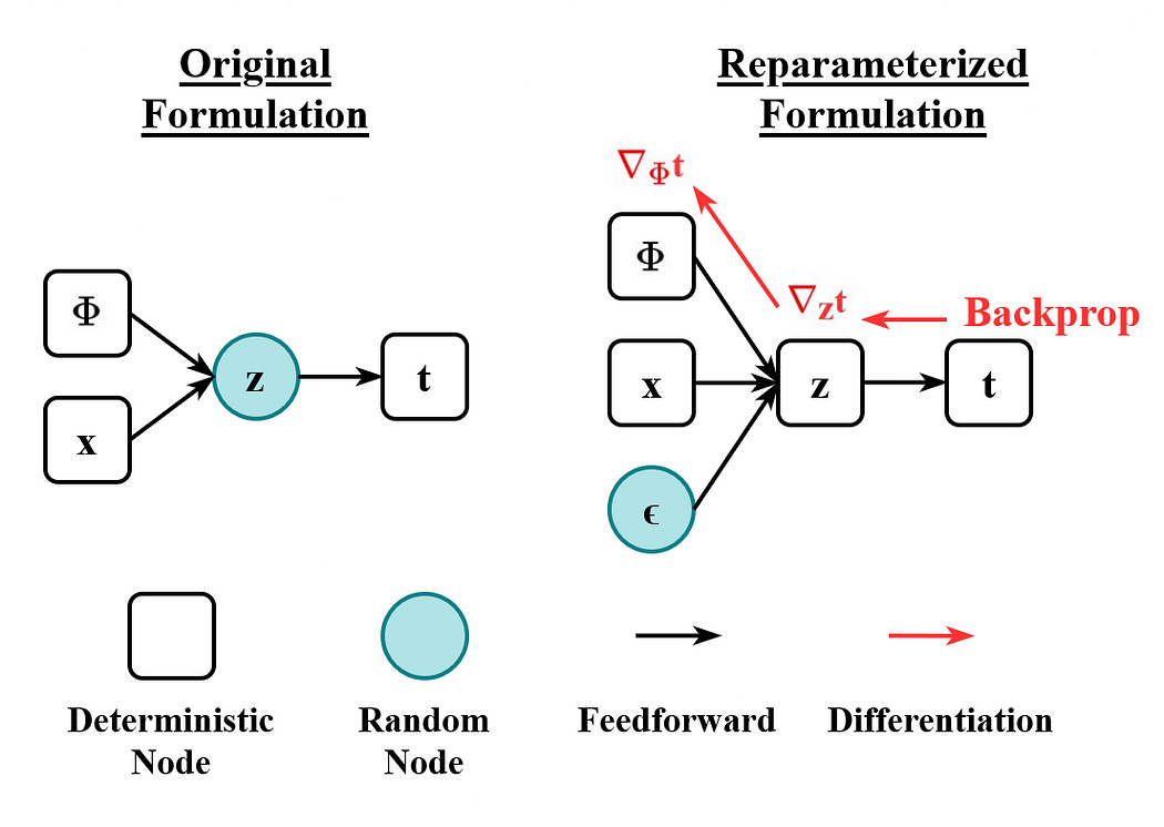
This might seem like a silly distinction because the result is fundamentally the same. Critically, though, it means the operation of sampling happens outside the model, which preserves differentiability. This seems like a great contender for a By-Hand article, so we’ll leave it as a high-level intuition for now.

Once we’ve sampled from our defined distributions, using the reparameterization trick to preserve differentiability, We can then compute the “log probability” between the output of our decoder, and our original input.

The math describing this is much more complex than it really has to be. This is essentially your basic loss function, like mean squared error or cross-entropy, just like what you would typically use in a typical regression or classification problem. I’ll cover those in-depth in a future article, but this is basically saying “If the reconstruction is right, spit out a big number. If it’s wrong, spit out a small number”.

All that’s left, really, is to understand the summation. In theory, you could do the reparameterization trick a few times by sampling a few points. Here, L is the number of points you sampled, where the loss is computed as the average (Adding up all the values with the summation ∑ and dividing by the number of samples L )

The KL Divergence, on the other hand, iterates through J , representing the size of the latent dimension between the encoder and the decoder. In other words, we’re calculating the KL Divergence across all of the distributions and adding them up.

So, we skimmed through some stuff, but I think we have a solid conceptual understanding of the VAE and how it relates to the loss function. The VAE encoder spits out distributions.

These then get sampled via the reparameterization trick and passed through the decoder to create a reconstruction.

Then, we calculate loss by penalizing the model for having distributions that deviate too far from a classic normal distribution with a mean of zero and a standard deviation of one. We also penalize the model for incorrect re-constructions. We then update the model to, in this case, maximize the loss function, which forces the model to find an overlapping set of distributions that still result in good re-constructions.

I say we go ahead and code it up!

Implementing a Variational Autoencoder

For all the theory, the implementation of a VAE is pretty straightforward. Here‘s defining a VAE and training it in under 80 lines of code:

import torch import torch.nn as nn import torch.nn.functional as F import torchvision from torchvision import transforms from torch.utils.data import DataLoader import matplotlib.pyplot as plt  # Load MNIST transform = transforms.ToTensor() train_dataset = torchvision.datasets.MNIST(root='./data', train=True, transform=transform, download=True) train_loader = DataLoader(train_dataset, batch_size=128, shuffle=True)  # Define VAE Model class VAE(nn.Module):     def __init__(self):         super().__init__()         # Encoder         self.encoder_core = nn.Sequential(             nn.Linear(28*28, 128),             nn.ReLU(True),             nn.Linear(128, 64),             nn.ReLU(True)         )         self.fc_mu = nn.Linear(64, 32)         self.fc_logvar = nn.Linear(64, 32)          # Decoder         self.decoder = nn.Sequential(             nn.Linear(32, 64),             nn.ReLU(True),             nn.Linear(64, 128),             nn.ReLU(True),             nn.Linear(128, 28*28),             nn.Sigmoid()         )      def reparameterize(self, mu, logvar):         std = torch.exp(0.5 * logvar)         eps = torch.randn_like(std)         return mu + eps * std      def forward(self, x):         x = x.view(x.size(0), -1)         h = self.encoder_core(x)         mu = self.fc_mu(h)         logvar = self.fc_logvar(h)         z = self.reparameterize(mu, logvar)         decoded = self.decoder(z)         return decoded.view(x.size(0), 1, 28, 28), mu, logvar  # Loss Function def vae_loss(recon_x, x, mu, logvar):     recon_loss = F.binary_cross_entropy(recon_x.view(x.size(0), -1), x.view(x.size(0), -1), reduction='sum')     kl_div = -0.5 * torch.sum(1 + logvar - mu.pow(2) - logvar.exp())     return recon_loss + kl_div  # Setup device = torch.device('cuda' if torch.cuda.is_available() else 'cpu') model = VAE().to(device) optimizer = torch.optim.Adam(model.parameters(), lr=1e-3)  # Training Loop epochs = 10 for epoch in range(epochs):     model.train()     total_loss = 0     for imgs, _ in train_loader:         imgs = imgs.to(device)         optimizer.zero_grad()         recon, mu, logvar = model(imgs)         loss = vae_loss(recon, imgs, mu, logvar)         loss.backward()         optimizer.step()         total_loss += loss.item()          avg_loss = total_loss / len(train_loader.dataset)     print(f"Epoch [{epoch+1}/{epochs}] Loss: {avg_loss:.4f}")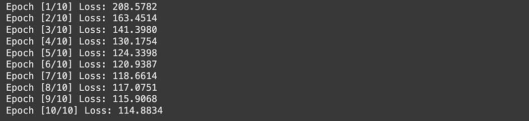

This is remarkably similar to the traditional autoencoder but with a few key differences. First of all, we have some new parameters. These project the output of the encoder into two vectors, one representing the mean and one representing the deviation.

self.fc_mu = nn.Linear(64, 32) self.fc_logvar = nn.Linear(64, 32)

Here, we output the mean directly, but we don’t actually output the standard deviation directly. Instead, we output the logvar (log variance), which is equal to log(σ²) , where σ is the standard deviation. This is convenient as the standard deviation of a value can never be less than or equal to zero, but neural networks like to output both negative and positive numbers. log(σ²) can be negative or positive, and then that can be used to calculate sigma.

Logvar can be converted to σ given the following expression:

So, back to the code, the encoder outputs the mean and logvar (which is, essentially, the standard deviation). When we pass our input through the variational autoencoder via the forward function, we pass the data to the encoder, then project the resulting vector into a vector of means and logvars. These then get passed through the reparameterize function to calculate a sample from the distributions.

x = x.view(x.size(0), -1) h = self.encoder_core(x) mu = self.fc_mu(h) logvar = self.fc_logvar(h) z = self.reparameterize(mu, logvar)

The reparameterize function contains the reparameterization trick. It first calculates the standard deviation from logvar, then samples a normal distribution to create some random point. That random point is then scaled by the standard deviation generated by the model, and shifted by the mean. This is happening in PyTorch, so these are vectorized operations which are happening in parallel. In this case, 32 times, as this particular model has 32 mu and logvar values per input. We then get a vector of values as the output.

def reparameterize(self, mu, logvar):   std = torch.exp(0.5 * logvar)   eps = torch.randn_like(std)   return mu + eps * std

This output is then passed to the decoder, which generates the reconstruction. The mu and logvar are also returned from the forward function, as those are required for calculating KL divergence loss.

decoded = self.decoder(z) return decoded.view(x.size(0), 1, 28, 28), mu, logvar

The actual loss function is as we described previously. There’s a part for KL divergence and another part for reconstruction loss. These are added together.

# Loss Function def vae_loss(recon_x, x, mu, logvar):     recon_loss = F.binary_cross_entropy(recon_x.view(x.size(0), -1), x.view(x.size(0), -1), reduction='sum')     kl_div = -0.5 * torch.sum(1 + logvar - mu.pow(2) - logvar.exp())     return recon_loss + kl_div

One important note, this is the negative of what is described in the paper. PyTorch expects a loss function where the objective is minimization, not maximization, so this particular loss function is multiplied by -1.

Anywho, we then train our model like any other model in PyTorch. Give it some data, calculate loss, update, repeat.

# Setup device = torch.device('cuda' if torch.cuda.is_available() else 'cpu') model = VAE().to(device) optimizer = torch.optim.Adam(model.parameters(), lr=1e-3)  # Training Loop epochs = 10 for epoch in range(epochs):     model.train()     total_loss = 0     for imgs, _ in train_loader:         imgs = imgs.to(device)         optimizer.zero_grad()         recon, mu, logvar = model(imgs)         loss = vae_loss(recon, imgs, mu, logvar)         loss.backward()         optimizer.step()         total_loss += loss.item()          avg_loss = total_loss / len(train_loader.dataset)     print(f"Epoch [{epoch+1}/{epochs}] Loss: {avg_loss:.4f}")

We can play around with our VAE and see that, once it’s been trained, it can indeed re-construct images.

# Visualize n reconstructions def visualize_vae_output(model, dataset, n=6):     model.eval()     dataloader = DataLoader(dataset, batch_size=n, shuffle=True)     imgs, _ = next(iter(dataloader))     imgs = imgs.to(device)      with torch.no_grad():         recon, _, _ = model(imgs)      fig, axes = plt.subplots(nrows=n, ncols=2, figsize=(5, 2 * n))     for i in range(n):         axes[i, 0].imshow(imgs[i].cpu().squeeze(), cmap='gray')         axes[i, 0].set_title("Original")         axes[i, 0].axis('off')          axes[i, 1].imshow(recon[i].cpu().squeeze(), cmap='gray')         axes[i, 1].set_title("Reconstruction")         axes[i, 1].axis('off')      plt.tight_layout()     plt.show()  # Call this after training visualize_vae_output(model, train_dataset)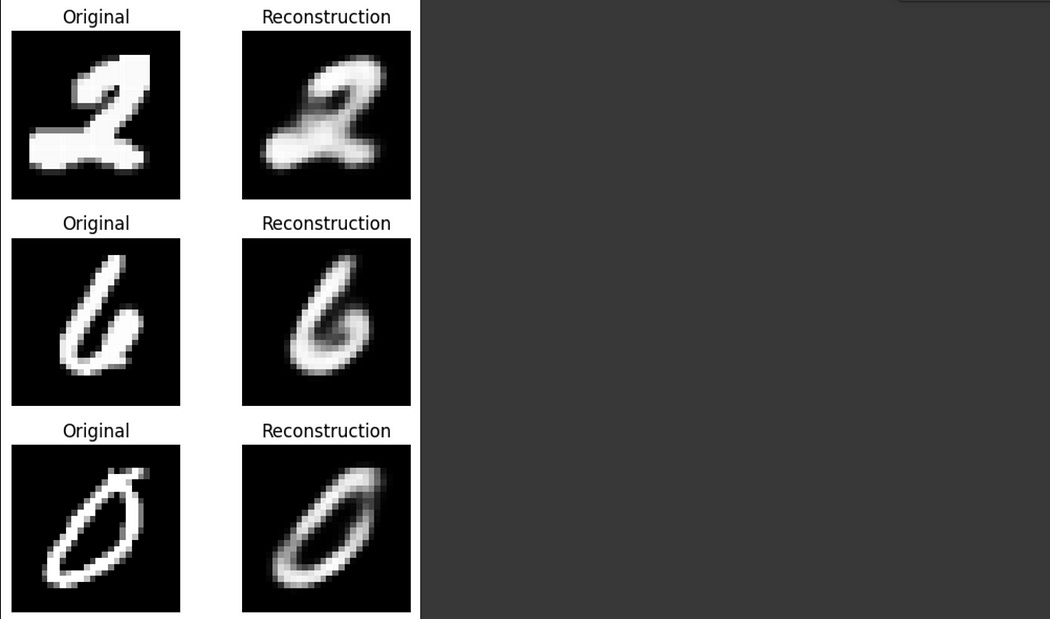

More importantly, though, we can explore the latent space itself, which is the whole point of the VAE. In the previous VAE, our latent space had a dimension of 32, but that’s hard to visualize. Here, with a few modifications, I’m training a VAE that has a latent dimension of two

import torch import torch.nn as nn import torch.nn.functional as F import torchvision from torchvision import transforms from torch.utils.data import DataLoader import matplotlib.pyplot as plt import numpy as np  # Set device device = torch.device('cuda' if torch.cuda.is_available() else 'cpu')  # Load MNIST transform = transforms.ToTensor() train_dataset = torchvision.datasets.MNIST(root='./data', train=True, transform=transform, download=True) train_loader = DataLoader(train_dataset, batch_size=128, shuffle=True)  # Define VAE with 2D latent space class VAE(nn.Module):     def __init__(self):         super().__init__()         # Encoder         self.encoder_core = nn.Sequential(             nn.Linear(28*28, 128),             nn.ReLU(True),             nn.Linear(128, 64),             nn.ReLU(True)         )         self.fc_mu = nn.Linear(64, 2)       # 2D latent         self.fc_logvar = nn.Linear(64, 2)          # Decoder         self.decoder = nn.Sequential(             nn.Linear(2, 64),               # match 2D latent             nn.ReLU(True),             nn.Linear(64, 128),             nn.ReLU(True),             nn.Linear(128, 28*28),             nn.Sigmoid()         )      def reparameterize(self, mu, logvar):         std = torch.exp(0.5 * logvar)         eps = torch.randn_like(std)         return mu + eps * std      def forward(self, x):         x = x.view(x.size(0), -1)         h = self.encoder_core(x)         mu = self.fc_mu(h)         logvar = self.fc_logvar(h)         z = self.reparameterize(mu, logvar)         decoded = self.decoder(z)         return decoded.view(x.size(0), 1, 28, 28), mu, logvar  # Loss function def vae_loss(recon_x, x, mu, logvar):     recon_loss = F.binary_cross_entropy(recon_x.view(x.size(0), -1), x.view(x.size(0), -1), reduction='sum')     kl_div = -0.5 * torch.sum(1 + logvar - mu.pow(2) - logvar.exp())     return recon_loss + kl_div  # Train model model = VAE().to(device) optimizer = torch.optim.Adam(model.parameters(), lr=1e-3)  epochs = 10 for epoch in range(epochs):     model.train()     total_loss = 0     for imgs, _ in train_loader:         imgs = imgs.to(device)         optimizer.zero_grad()         recon, mu, logvar = model(imgs)         loss = vae_loss(recon, imgs, mu, logvar)         loss.backward()         optimizer.step()         total_loss += loss.item()          avg_loss = total_loss / len(train_loader.dataset)     print(f"Epoch [{epoch+1}/{epochs}] Loss: {avg_loss:.4f}")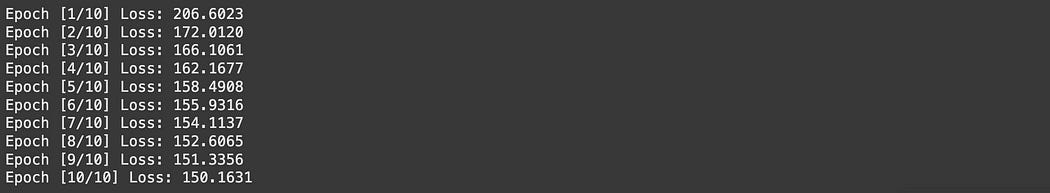

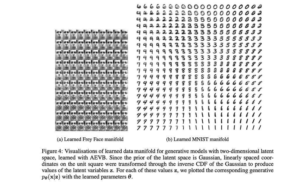
This is convenient because it makes visualization easy. We can traverse through points in a 2D space, and use those as latent representations. We can then see what our VAE decoder generates as an output.

def plot_latent_manifold(model, grid_size=20, range_lim=3):     model.eval()      with torch.no_grad():         # Create 2D grid of latent vectors         z_grid = torch.tensor([             [x, y]             for y in np.linspace(-range_lim, range_lim, grid_size)             for x in np.linspace(-range_lim, range_lim, grid_size)         ], dtype=torch.float32).to(device)          # Decode to images         generated = model.decoder(z_grid).view(-1, 28, 28).cpu().numpy()      # Plot grid of images     fig, axes = plt.subplots(grid_size, grid_size, figsize=(8, 8))     for i in range(grid_size):         for j in range(grid_size):             ax = axes[i, j]             ax.imshow(generated[i * grid_size + j], cmap="gray")             ax.axis("off")     plt.tight_layout()     plt.show()  # After training, visualize manifold plot_latent_manifold(model)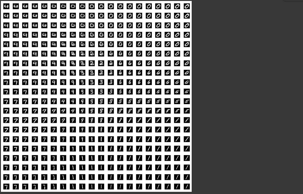

As you can see, our VAE has learned to organize representations in a way where features blend between one another. 0 blends into 4 and 6 due to their shared round qualities, 1 blends smoothly to 7, and to 5. 8 and 9 blend between each other, and 9 and 7 blend between one another.

Here, we’re forcing all of the numbers in MNIST to be represented with just two values, which we’re plotting on the x and y axis, but one could imagine, that with higher dimensions, the model might learn even better and more intuitive forms of organization. instead of 1–7 being a region in the space, it might be relegated to an entire dimension.

This smoothness is incredibly helpful in creating variational autoencoders that are useful to data scientists, as well as machine learning models. because the encoder can take any MNIST image and turn it into this smooth space, it’s very easy to plug some other AI model into it, such that that AI model can leverage that robust representation to do something else.

This is pretty spiffy and would be worth concluding on within itself, but there’s one other topic I want to discuss.

Disentangled Variational Autoencoders

Don’t worry, variational autoencoders comprise the vast majority of the theory of this article. Disentanglement, really, is just a minor modification of the fundamental VAE recipe.

A Disentangled VAE is just like a normal VAE, but with one number added to it, a hyperparameter β (Beta). For this reason, disentangled variational autoencoders are often abbreviated as “β-VAEs”. Instead of the traditional variational autoencoder we previously discussed, which has a loss function like so:

β-VAEs scale the KL divergence by a parameter Beta

Typically β is either greater than or equal to 1. When β is equal to 1, we just have a classic variational autoencoder. However, when β is greater than one, the effects of KL divergence take a greater effect.

Recall, in our original loss function, that we sum over all of the deviations when calculating KL divergence.

When the penalty for KL divergence is increase, the variational autoencoder is more disincentivized to create distributions that deviate from a mean of zero and sa tandard deviation of 1. Thus, β-VAEs like to make as few distributions as possible which actually encode the information. Practically, this makes β-VAEs much more likely to encode very high-level information within the latent space. When β-VAEs are applied to images of faces, for instance, they’re likely to encode very human interpretable information in their dimensions, like rotation, smiling, light direction, ethnicity, etc. This is because, even if a β-VAE can encode more subtle information across multiple spots in the latent space, it’s heavily incentivized not to, and to instead encode information via very high-level features that are broadly applicable.

To actually implement a β-VAE, it’s as easy as adding the β to our VAE and training it. This particular β-VAE has a latent dimension of 8.

latent_dim = 8  import torch import torch.nn as nn import torch.nn.functional as F import torchvision from torchvision import transforms from torch.utils.data import DataLoader import matplotlib.pyplot as plt import numpy as np  # Set device device = torch.device('cuda' if torch.cuda.is_available() else 'cpu')  # Load MNIST transform = transforms.ToTensor() train_dataset = torchvision.datasets.MNIST(root='./data', train=True, transform=transform, download=True) train_loader = DataLoader(train_dataset, batch_size=128, shuffle=True)  # Define Beta-VAE with 4D latent space class BetaVAE(nn.Module):     def __init__(self, latent_dim=4):         super().__init__()         self.latent_dim = latent_dim          # Encoder         self.encoder_core = nn.Sequential(             nn.Linear(28*28, 128),             nn.ReLU(True),             nn.Linear(128, 64),             nn.ReLU(True)         )         self.fc_mu = nn.Linear(64, latent_dim)         self.fc_logvar = nn.Linear(64, latent_dim)          # Decoder         self.decoder = nn.Sequential(             nn.Linear(latent_dim, 64),             nn.ReLU(True),             nn.Linear(64, 128),             nn.ReLU(True),             nn.Linear(128, 28*28),             nn.Sigmoid()         )      def reparameterize(self, mu, logvar):         std = torch.exp(0.5 * logvar)         eps = torch.randn_like(std)         return mu + eps * std      def forward(self, x):         x = x.view(x.size(0), -1)         h = self.encoder_core(x)         mu = self.fc_mu(h)         logvar = self.fc_logvar(h)         z = self.reparameterize(mu, logvar)         decoded = self.decoder(z)         return decoded.view(x.size(0), 1, 28, 28), mu, logvar  # Loss function with beta def beta_vae_loss(recon_x, x, mu, logvar, beta=4.0):     recon_loss = F.binary_cross_entropy(recon_x.view(x.size(0), -1), x.view(x.size(0), -1), reduction='sum')     kl_div = -0.5 * torch.sum(1 + logvar - mu.pow(2) - logvar.exp())     return recon_loss + beta * kl_div    # Train model model = BetaVAE(latent_dim=latent_dim).to(device) optimizer = torch.optim.Adam(model.parameters(), lr=1e-3)  epochs = 10 for epoch in range(epochs):     model.train()     total_loss = 0     for imgs, _ in train_loader:         imgs = imgs.to(device)         optimizer.zero_grad()         recon, mu, logvar = model(imgs)         loss = beta_vae_loss(recon, imgs, mu, logvar, beta=4.0)         loss.backward()         optimizer.step()         total_loss += loss.item()          avg_loss = total_loss / len(train_loader.dataset)     print(f"Epoch [{epoch+1}/{epochs}] Loss: {avg_loss:.4f}")

notice that the loss function returns recon_loss + beta * kl_div. Here, beta = 4, meaning this β-VAE penalizes distributions that deviate from a standard distribution four times more than a traditional VAE.

We can then visualize some of these latent dimensions. Here I’m creating a vector [0,0,0,0,0,0,0,0] and experimenting with the effects of modifying each one of these dimensions individually.

# Enhanced latent traversal visualization import torch import matplotlib.pyplot as plt  model.eval() with torch.no_grad():     steps = 11  # number of interpolation steps     z_range = torch.linspace(-3, 3, steps).to(device)     base_z = torch.zeros(1, latent_dim).to(device)      fig, axes = plt.subplots(latent_dim, steps, figsize=(steps * 1.5, 6))          for dim in range(latent_dim):  # for each latent dimension         for i, val in enumerate(z_range):             z_mod = base_z.clone()             z_mod[0, dim] = val             img = model.decoder(z_mod).view(28, 28).cpu().numpy()             ax = axes[dim, i]             ax.imshow(img, cmap='gray')             ax.axis('off')             if dim == 0:                 ax.set_title(f"{val:.1f}", fontsize=8)          axes[dim, 0].set_ylabel(f"z[{dim}]", rotation=0, labelpad=15, size=12, ha='right', va='center')      plt.suptitle(f"β-VAE Latent Space Traversal ({latent_dim}D)", fontsize=16)     plt.tight_layout()     plt.subplots_adjust(top=0.88)     plt.show()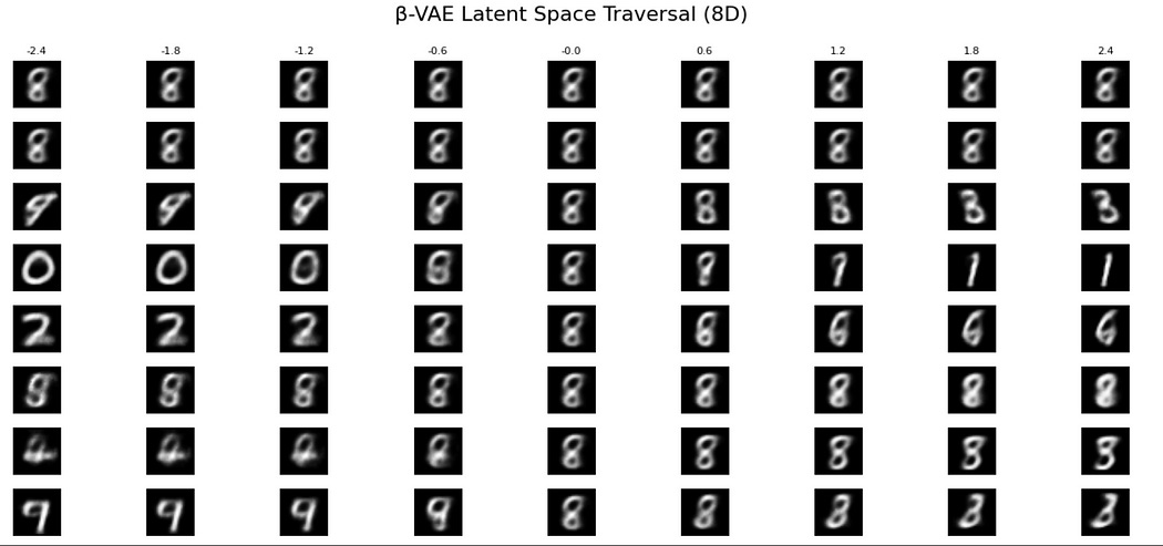

As you can see, it appears the first two dimensions do pretty much nothing, likely because the β-VAE decided that six dimensions were enough.

It appears “8” is at the center of all distributions, which kind of makes sense if you think about it. 7-segment displays are based around 8, so it’s kind of cool that our β-VAE appears to be doing the same thing.

As we modify some of the dimensions:

• The third dimension seems to interpolate between 9-ness 8-ness, and 3-ness.

• The fourth dimension appears to interpolate between hole characteristics, thus encoding 0–8–1

• The fifth dimension appears to encode 2–6 ness, which kind of makes sense, to me at least.

• The sixth dimension appears subtle, it may have some interdependence with other dimensions, but I’m seeing what looks like 5-ness going on in the left-hand side

• In the seventh and 8th dimensions, I’m seeing some 3-ness, 4-ness, and 7-ness.

These features are still a bit vague, but as you can see, there are some fairly defined characteristics encoded in just a few dimensions that have some degree of interpretability. This makes β-VAE more useful in some tasks than VAEs, and much much more useful in some tasks than traditional autoencoders.

Conclusion

I hope you learned a thing or two, I sure did!

In this article we discussed autoencoders. We started with the traditional autoencoder, then built up a modification of autoencoders to make their latent representations more useful in the form of variational autoencoders. We spent a fair amount of time there, building up the mathematical intuition of VAEs, and ultimately implemented one from scratch. We then used our knowledge of VAEs to implement a β-VAE, which is very similar to a normal VAE, but with a subtle modification to encourage higher level and arguably more useful features.

Stay tuned, now that I’ve discussed autoencoders, I have a few pieces planned to describe their applications!

Intuitively and Exhaustively Explained